- Visualización y acceso a datos
- Layer data source
- Herramientas de consulta y descubrimiento
- Information tool
- Fast information tool
- Measuring areas
- Measuring distances
- Catalog. Searching for geodata
- Gazzeteer
- Hiperenlace avanzado
- Navigation tools
- Navigating arround/ exploring the view
- Configuring locator map
- Centring the view on a point
- Locate by attribute
- Loading data
- Geografic data
- Introduction
- Vectorial
- Adding a layer from a disk file
- Adding a layer using the WFS protocol
- Introduction
- Connecting to the server
- Accessing to the service
- Selecting 'layers'
- Selecting 'attributes'
- 'Options' tab
- Filter
- Adding the layer to the view
- Modifying the layer's properties
- Filtrado por área
- Adding a layer using vectorial ArcIMS protocol
- Introduction to ArcIMS
- Connecting to image services
- Adding a layer using ArcIMS protocol
- Introduction
- Connecting to the server
- Accesing the service
- Selecting layers
- Adding the layer to the view
- Points to remember about spatial reference systems
- Modifying layer's properties
- Information about scale limits
- Attribute information request
- Connecting to geometry services
- Adding a geometry layer
- ArcIMS symbols
- Symbos
- Legends
- Working with the layer
- Raster
- Adding a layer from a disk file
- Adding a layer usins WMS protocol
- Introduction
- Connecting to the server
- Accessing to the service
- Selecting 'layers'
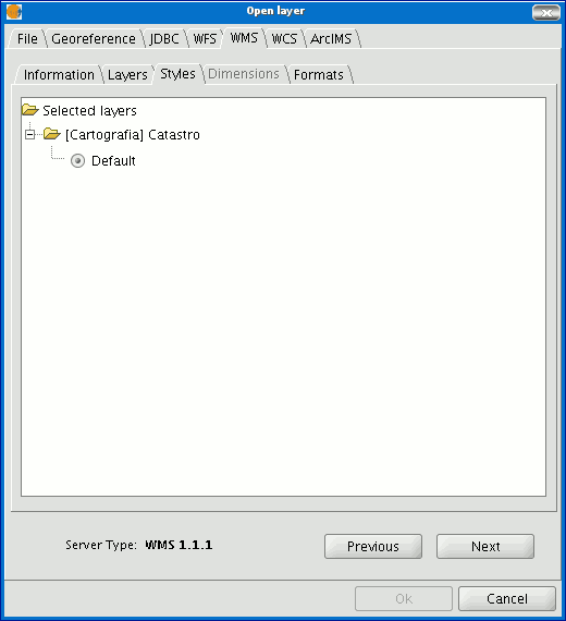
- Selecting 'styles'
- Selecting values for a WMS layer's 'dimensions'
- Selecting the format, spatial system and/or transparency
- Adding the WMS layer to the view
- Modifying the layer's properties
- Adding a layer using WCS protocol
- Introduction
- Accesing to the service
- Selecting 'Coverages'
- Selecting 'Format'
- Adding WCS layer to the view
- Modifying the layer's properties
- Adding orthophotos using the ECWP protocol
- Adding a layer using raster ArcIMS protocol
- Introduction to ArcIMS
- Connecting to image services
- Adding a layer using ArcIMS protocol
- Introduction
- Connecting to the server
- Accesing the service
- selecting layers
- Adding the layer to the view
- Points to remember about spatial reference systems
- Modifying layer's properties
- Information about scale limits
- Attribute information request
- Connecting to geometry services
- Adding a geometry layer
- ArcIMS symbols
- Symbols
- Legends
- Working with the layer
- Web Map Context
- Alfanumeric
Visualización y acceso a datos
Layer data source
Different types of cartographic information can be added to a view. Vector and raster files can be loaded. Each of these groups can contain a wide range of formats.
GIS data: The standard GIS format is the shape, which stores both spatial data and their attributes. A shape (also called “Shape file”) is actually three or more files with the same name and different extensions (even though in gvSIG it is handled as one file):
dbf: Table of attributes.
shp: Spatial data.
shx: Spatial data index.
From version 0.5 onwards, gvSIG also has the capacity to access the MySQL Spatial and PostGIS spatial data bases via a new driver which uses JDBC.
CAD data: These are vector drawing files which support the dxf and dgn formats. The CAD files may contain information on points, lines, polygons and texts. From version 0.4 onwards, gvSIG also allows access to the information contained in Autodesk’s 2000 dwg files.
WMS data (Web Mapping Service): gvSIG can be used to consult WMS data, i.e. data available on the web. WFS data (Web Feature Service): From version 0.5 onwards, gvSIG can be used to download WFS vector layers from servers that comply with the Open Geospatial Consortium (OGC) Standard.
WCS data (Web Coverage Service): From version 0.4 onwards, gvSIG allows access to remote information based on the OGC’s WCS protocol.
GML (Geography Markup Language): From version 1.0 onwards, gvSIG allows GML documents to be displayed and exported. Geography Markup Language (GML) is an XML format to transport and store geographic information whose design is based on specifications produced by the OGC group.
Images: gvSIG can display different raster images (tiff, jpg, ecw, mrsid, etc.). From version 0.4 onwards, gvSIG can save images which have been modified in these formats.
From version 0.5 onwards, “colour palette” (GIFs, 8-bit PNGs, etc.) raster files can be opened and raster files without georeferencing can also be opened. Moreover, this new version supports GIF, BMP y JPEG2000 formats.
Herramientas de consulta y descubrimiento
Information tool
You can access the information tool via the following button in the tool bar

or by going to the “View” menu bar, to “Query” and then to “Information”.
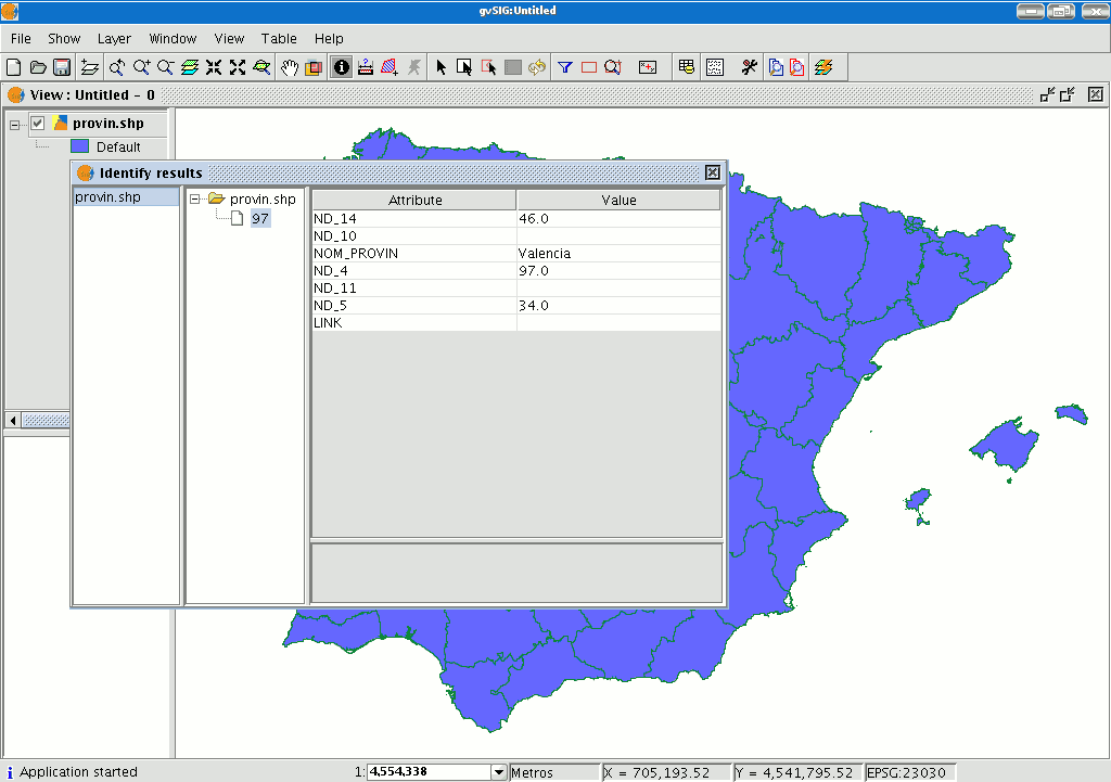
The “Information Tool” is used to obtain information about the map elements.
When you click on an element using this tool, gvSIG shows the selected element’s attributes in a dialogue window. However, the layer of the element you wish to identify must previously be activated.
Fast information tool
In gvSIG, this tool is used to quickly display available information when working with a view containing visible vector layers (including WFS layers, which are vector layers).
 Quick Info is enabled if vector layers are visible in the current view.
 Quick Info is disabled if no vector layers are visible in the current view.
With this tool you can select fields from vector layers visible in the current view. Information from these fields is displayed as you move the mouse cursor over the view. The tool works in combination with any other tools selected for the view.
You can access the Quick Info tool in two ways:
- Via the menu: View → Query → Quick Info
- Via the icon on the toolbar.
When the tool is selected a progress bar is displayed which shows the layers being loaded:
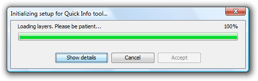
Progress bar for loading information
If there were no problems loading the information the Quick info field selection dialog is shown:
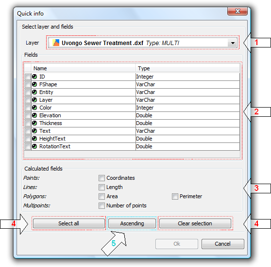
Dialog for the selection of fields
- Drop-down list for selecting vector layers. Lists the layers in the order that they appear in the TOC of the active view. The following information is shown:
Level of the Layer in the TOC: displays icons and grouping nodes  containing the layer. The last icon always represents the vector layer.
Name of the layer.
Type of geometry of the layer: five types of geometry layer are supported: point, line, polygon, multipoint, and multi (the latter may contain any of the above).
- List of Fields. Contains three columns:
- Selection box (checkbox): indicates whether or not to display the field information.
- Field Type + Field Name: the field type is represented by an icon as shown in the following table:
 The field type is simple.
- The field type is complex.
- Type of field: according to the SQL types.
- Calculated fields. List of checkboxes to select which geometry fields to calculate. These vary depending on the geometry of the layer:
- Point layer: point coordinates.
- Line layer: length of the line.
- Polygon layer: perimeter and area of the polygon.
- Multipoint layer: number of points.
- Multi-geometry layer: any of the above; the information will vary according to the selection and the nature of the geometry.
 The units of length and area are displayed using the measurement units of the View.
- Selecting / de-selecting all the fields in the layer. Select or de-select all the fields in the layer.
- Sort fields. Sort fields alphabetically in ascending or descending order, or according to the internal order of the layer (default).
After selecting the fields, click Ok to enable the tool in the current view. The Quick info tool works in combination with Quick info tools for other Views. Thus, when enabled, it combines with each active View to display information. The tool settings can be changed for each View and are linked to that View.
As the cursor is moved over the geometry of a layer, the information box showing the information is displayed and/or updated. This box disappears when the cursor no longer "points" to any geometry of the layer.
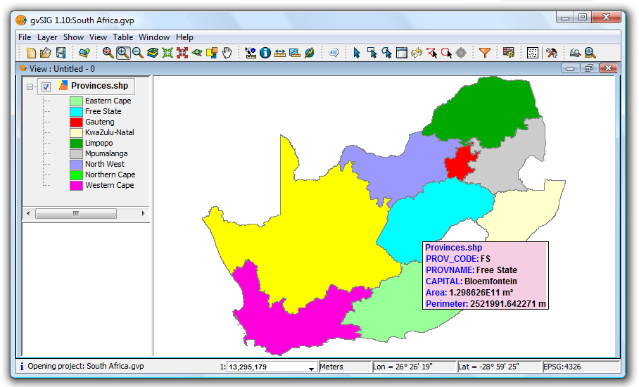
Example showing the display from the Quick info tool
If there is more than one geometry adjacent to the point indicated by the cursor then information is displayed about all of them, as distinguished by the unique internal identifier of the geometry.
Thus, the information is provided in the following order:
- Name of the layer.
- Information on the geometry (for each one):
ID: unique identifier of the geometry in the data source layer (optional, only visible if you have information on more than one geometry).
Selected fields: those fields selected to display layer information.
Optional fields: those calculated fields selected from the geometries of the layer.
 It should be noted that currently gvSIG adds the area and perimeter of islands to the geometry containing them.
Measuring areas
You can access this tool via the following button

or by going to the “View” menu and then to “Query” and “Measure area”.
This tool works in much the same way as “Measure distances”. Click on the point that represents the first polygon vertex that defines the area to be measured. Move the mouse and click on each new vertex until you reach the last one, then double click so that the application knows there are no more.
The calculation for the measured area appears at the bottom right of the view window.

Measuring distances

This tool provides information about the distance between two points. You can also access the tool by going to the “View” menu, to “Query” and then to “Measure distances”.

Firstly, make sure you have correctly defined the units of measurement (metres by default).
Remember that the units can be defined in the “Project manager” in the view properties or from the “View” menu and the “Properties” when working in a view.
You can use the measure distance tool by clicking on the mouse at the source point and dragging it to the destination point.
You can take as many measurements as you like. Double click on the last one to finish.
The calculation for the measured distance appears at the bottom of the view window. Both the distance of the last measured segment and the total distance are shown.
Catalog. Searching for geodata
Introduction
The catalogue service allows you to search for geographic information on the Internet. gvSIG offers a user-friendly interface which allows you to find geodata and load it in the view, as long as the nature of the data allows this.
Connecting to a server
Before you can carry out a search, you will need to connect to a catalogue server. To access the wizard, you will first need to open a view and then click on the following button:

The first window of the catalogue opens. Input the required parameters to connect to a server. These include:
- The server address.
- The server protocol, which in the case of the catalogue can be:
- Z39.50: General information retrieval protocol.
- SRU/SRW: Variant of Z39.50.
- CSW: Catalogue protocol defined by the OGC in the “Catalogue Interface 2.0” specification.
- Data base name: You only need to indicate the data base you wish to connect to in the case of z39.50. If no value is input you will connect to the default data base.

Then click on the “Connect” button. If the connection is made and the server supports the specified protocol, a new window will appear to start the search.
Searching
To carry out a search, you need to fill in the fields that appear in the following form.
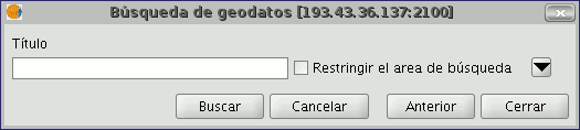
Click on the button and the window will drop down to show more fields which will allow you to carry out an advanced search. The fields you can search in are set by the server. This means that some of the search fields in this form may have no effect in some servers.
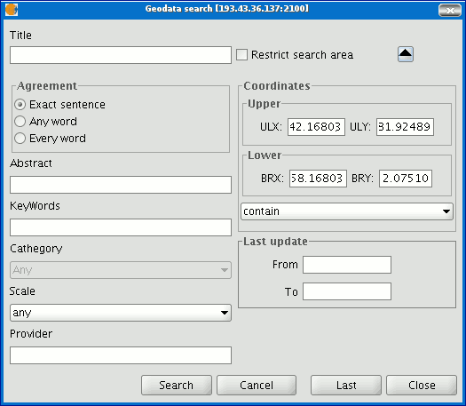
If you change the view zoom, the new coordinates will be reflected in this form. If you wish to restrict the search area enable the corresponding check box. Then click on “Search” and wait for the search to be carried out.
Viewing the results
If the search has been successful, a new window containing the search results will open.
Use the “Previous” and “Next” buttons to see each of the results obtained.
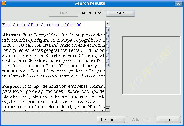
The left-hand side of the window shows information about the metadata obtained. If you wish to see all the information, click on the "Description" button.
You will also be able to see a miniature image at all times, metadata permitting.
If the metadata has any geodata associated to it, the “Add layer” button will be enabled.
gvSIG can currently recognise different types of associated resources, such as WMS, WCS, Postgis tables and web pages.
If you click on this button, a new window will be opened and will show all the resources the application has been able to find.
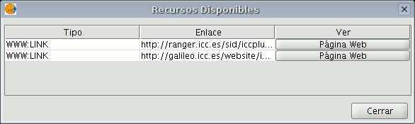
If you click on a WMS, WCS or Postgis type resource, the new layer will automatically be loaded in gvSIG. If the resource is a web page, for example, the operating system’s default browser.
Gazzeteer
Introduction
A gazetteer is a data set in which a link is established between a toponym and its geographic coordinates.
gvSIG has a catalogue client which allows you to search by toponyms and centre the view on a specific point.
Connecting to a server
Create a view first and open it. The following button will appear automatically in the gvSIG tool bar.

Click on the button. A wizard opens to help you to carry out a search. The parameters to be input are:
- The server address.
- The server protocol, which in the case of the gazetteer can be:
- WFS-G: Toponym search protocol defined by the OGC.
- WFS: Although this protocol was created with a different purpose in mind, it can be used for a toponym search, as long as it has a text attribute in one of the tables. This protocol also allows you to carry out a “Feature” search in any other field, but not necessarily a text attribute.
- ADL: Protocol specified by the Alexandria Digital Library.
- IDEC/SOAP: Protocol that uses the Catalonian Cartographic Institute (ICC) gazetteer web service.
When you have input all the parameters, click on the "Connect" button and wait until the server is found and accepts the specified protocol. If it is accepted, a new window will appear to start the search. If not, an error message will appear.
Searching
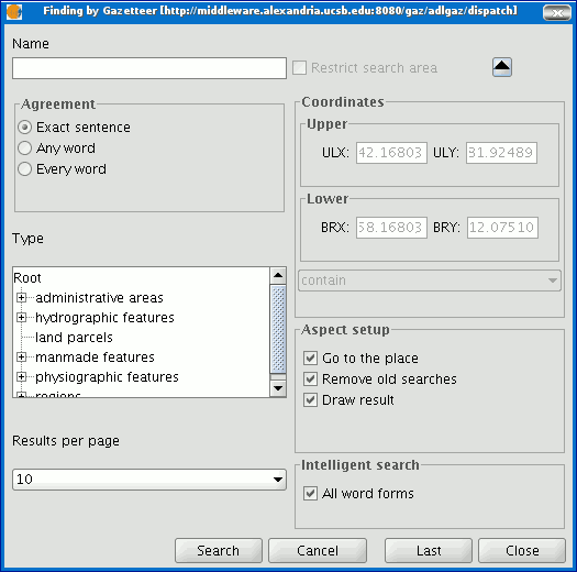
To carry out a search, you will need to fill in the criteria that appear in the following form. You can see the simplified form or carry out an advanced search by clicking on the button in the top right hand corner. This drops down the window.
If you change the view zoom, the new coordinates will be reflected in this form. If you wish to restrict the search area activate the corresponding check box. There are also three options in the “Aspect set up” box which you can use to set up the search view:
Zoom to search: This puts the toponym found in the centre of the gvSIG view.
Delete old searches: This deletes all the texts found in the previous searches from the view.
Draw result: This draws a point and a text label in the place the resulting toponym has been found.
When you have filled in all the fields in the form, click on “Search” and wait for the search to be carried out.
Viewing the results
A new window containing the search results will open. Use the “Previous” and “Next” buttons to move through the different pages of results.
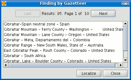
Finally, select the toponym required and click on “Localise”. The gvSIG view will centre on the point the toponym is located in.
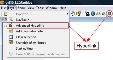
Hiperenlace avanzado
The Advanced Hyperlink tool in this version of gvSIG significantly extends the functionality of the hyperlink tool found in version 1.1.
The tool is accessible either from the Layer menu (Layer > Advanced Hyperlink) or by clicking the icon on the toolbar.
Accessing the Hyperlink tool
Hyperlinks are configured at the layer level, which means that they can be enabled or disabled per layer. To set the hyperlink for a layer, double-click on the layer name in the TOC to open the Layer Properties and select the Hyperlink tab.
The hyperlink configuration screen looks like this:
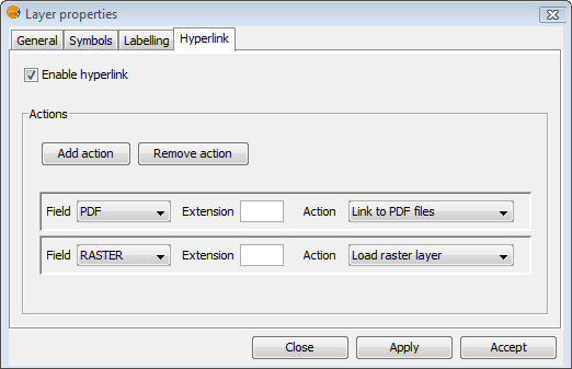
Hyperlink Configuration
Remember that the layer's attribute table must be correctly prepared for the hyperlinks to work. To do this, edit the relevant record and insert the path to the hyperlinked file, leaving out the extension.
After the hyperlinks have been setup and enabled, select the Advanced Hyperlink tool and find the item in the View that corresponds to the record associated with the link. Click on the item and a window will open displaying the linked file.
Actions
The Advanced Hyperlink tool provides the following actions:
- Link to text and HTML files: the tool will open a window in gvSIG and load the linked text or HTML document into it.
- Link to image files: the tool will open a window in gvSIG and load the linked image into it.
- Link to PDF files: the tool will open a window in gvSIG and load the linked PDF document into it.
- Load raster layer: the tool loads the raster layer into the active View.
- Load vector layer: the tool loads the vector layer into the active View.
- Link to SVG files: the tool will open a window in gvSIG and load the linked SVG file into it.
NOTE 1: When editing the hyperlink fields in the attribute table, if a path longer than the maximum field length is entered, the path will be truncated (without warning) to the maximum field length. By default, fields are created with a maximum length of 50 characters. Fields should be defined to handle long paths when necessary, otherwise only very short paths can be stored.
For example: if we enter
C:/Documents and Settings/My documents/images/villafafila.jpg
and the maximum field length is 50 characters, the path will be truncated to:
C:/Documents and Settings/My documents/images/vill
which is not what is wanted.
NOTE 2: Please note that if the path you enter contains an image or file extension that is registered in the registry, you should not also enter it when configuring the hyperlink properties as this would be duplicating the information.
Navigation tools
Navigating arround/ exploring the view
Navigating arround/ exploring the view
There are several tools you can use to navigate around the map. These are basically zooms and panning.
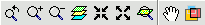
Zoom and panning
You can activate these tools by clicking on the "View” menu and then on “Navigation".
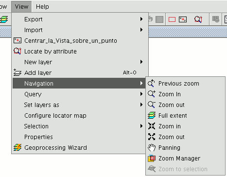
or by using the button bar which is quicker. Zoom in: Enlarges a particular area of the view.

Zoom out: Reduces a particular area of the view.

Previous zoom: Goes back to the previous zoom used.

Full extent: Full zoom of the total area included in all the layers of the view.

Panning: This allows you to change the view zoom by dragging the viewing field all over the view with the mouse. Click and hold down the left button of the mouse then move the mouse in the direction you require.

Zoom to selection: Full zoom of the total area of all the selected elements.

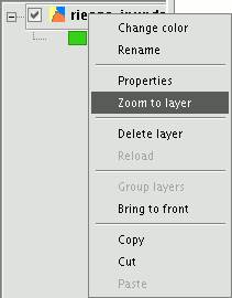
Zoom to layer: To zoom to the layer, right click on the selected layer in the ToC, or click on the “Zoom to layer” option in the contextual menu.
Zoom manager
You can access the “Zoom manager” from the tool bar by clicking on the following button:

or from the “View” menu, then “Navigation” and “Zoom manager”.
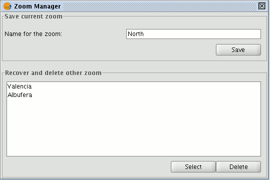
By clicking on the “Zoom manager” you can save a zoom so that you can go back to it at a later stage.
This tool can be used to name the current zoom of the view with the text bar which appears in the window.
Click on “Save” and the zoom currently in the view will automatically be added to the “Zoom manager” text box.
You can create and save as many zooms as you wish. Use the "Select” and “Delete” buttons to manage your working areas.
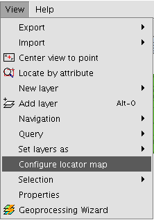
Configuring locator map
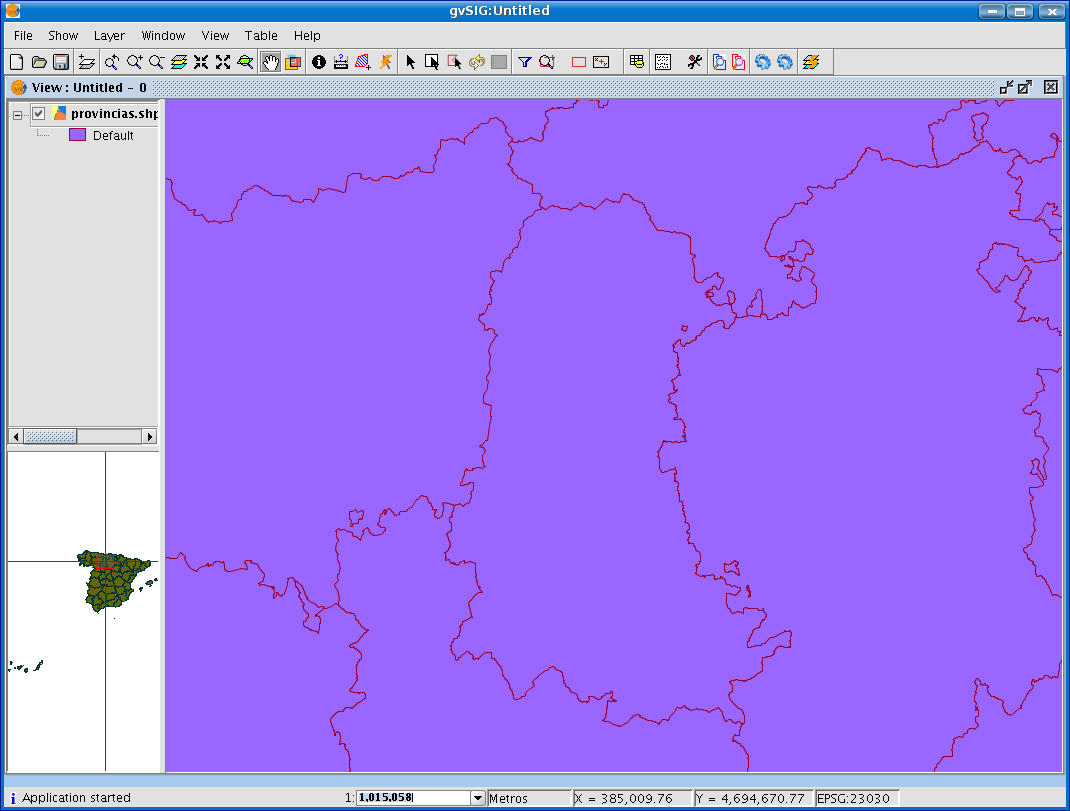
The locator is a general map which is displayed in the bottom left hand corner of the view's window. It is used to show the working area (main window zoom). Click on “View” in the menu bar and select “Configure locator map”.
A window appears in which we can add layers (we can add the same types of layers as in the view) which will make up part of the locator map. This window can also be used to remove layers or edit the layers’ legends.
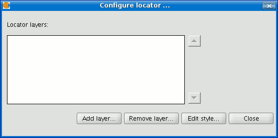
When you click on the “Add layer” button, the following window appears
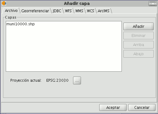
This new function allows the layer loaded in the locator map to be reprojected. To do this, click on the button next to “Current projection when you have selected the layer you wish to load in the locator map.
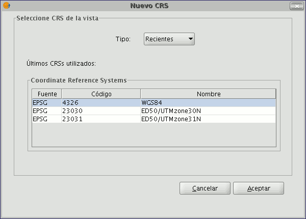
In the following window, select the reference system you wish the layer to have in the locator map and click on “Finish” for the changes to take effect.
Centring the view on a point
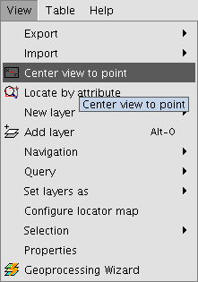
This tool allows you to locate a point in the view by its coordinates and to centre the view on this point.

You can also access the tool by going to the “View” menu then to “Centre view on a point”.
When you have accessed the tool, a dialogue box will appear in which you can input the required coordinates and select the point colour.
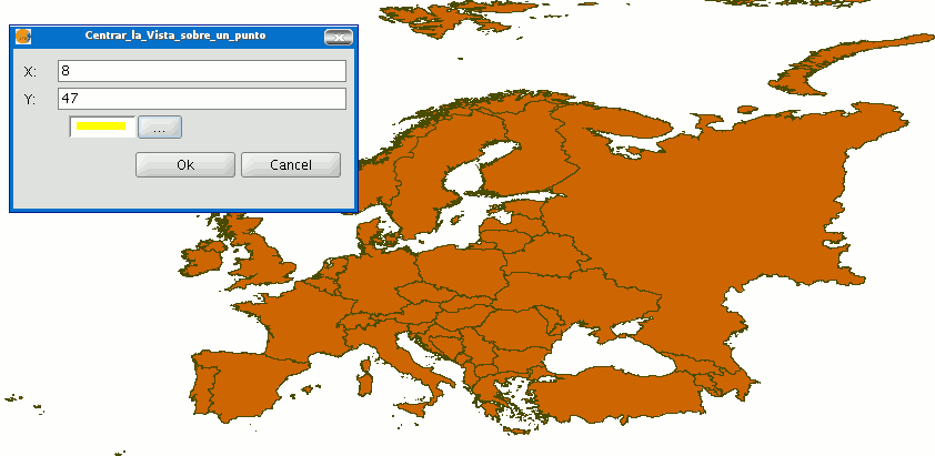
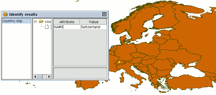
When you click on the "Ok" button, the view centres on this point and the information window that corresponds to this point appears.
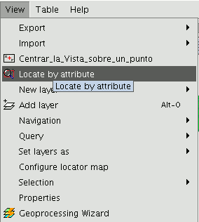
Locate by attribute
This tool allows you to zoom in on areas of a layer by specifying the value of a particular attribute. You can access this tool by clicking on the button

or by going to the “View” menu then to “Locate by attribute”.
When the tool is selected, the following window appears
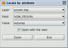
You will find all the layers loaded in the ToC in the “Layer” pull down menu. The fields associated with the chosen layer are included in the “Field” pull down menu.
The data included in the selected field appears in the "Value" pull down menu.
If you mark the “Open with the view” check box and decide to close the view, the “Locate by attribute” window will appear the next time you open the view.
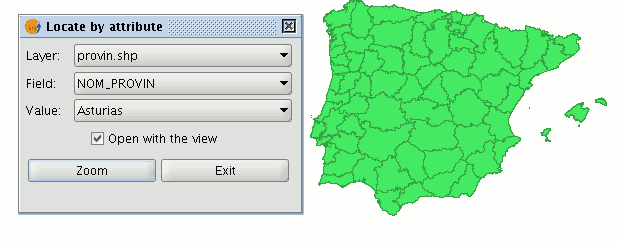
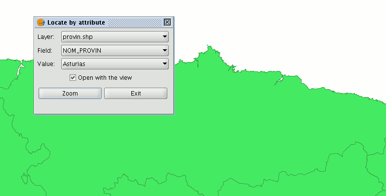
When you have made the selection, click on the "Zoom" button and the chosen area will be shown in the view.
Loading data
Geografic data
Introduction
Firstly, open a “View” document in gvSIG.
You can access this option by going to the "View" menu and then to "Add layer" or by using the “Control + O” key combination
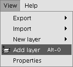
or by clicking on the "Add layer" button in the tool bar.

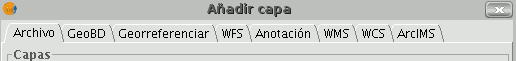
A window appears in which you can select and configure the layer's data source by its type:
Vectorial
Adding a layer from a disk file
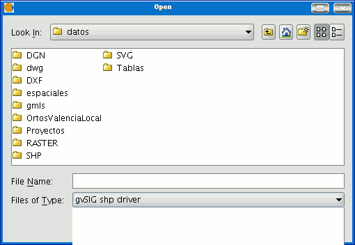
Click on the "Add" button
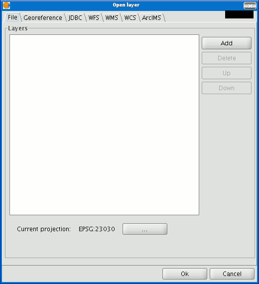
The "Add” dialogue window allows you to move around the file system to select the layer to be loaded. Remember that only the files of the type selected will be shown. To indicate the type of file to be loaded, select a file from the “Files of type” pull down menu.
If several layers are loaded at the same time, the order in which the themes will be added to the view can be specified with the "Up" and "Down" buttons in the “Add layer" dialogue.
Adding a layer using the WFS protocol
The Web Feature Service (WFS) is one of the OGC standards (http://www.opengeospatial.org) which is included in the list of standards (of this type) that gvSIG supports.
WFS is a communication protocol via which gvSIG retrieves a vector layer in GML format from a supporting server. gvSIG retrieves the geometries and attributes associated to each "Feature” and interprets the contents of the file.
Go to the “Add layer” and then select the WFS tab.
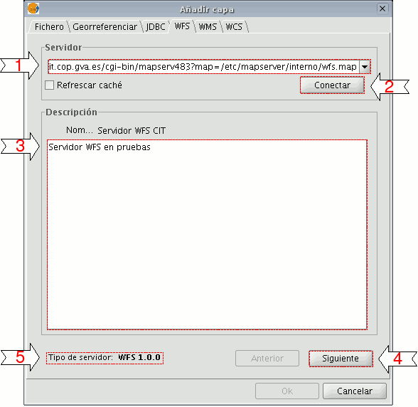
1. The pull-down menu shows a list of WFS servers (you can add a different server if you don’t find the one you want).
2. Click on “Connect”. gvSIG connects to the server.
3. and 4. When the connection is made, a welcome message from the server appears, if this has been configured. If no welcome message appears, you can check whether you have successfully connected to the server if the “Next” button is enabled.
5. The WFS version number that the server you have connected to is using is shown at the bottom of the box.
N.B. You can select the “Refresh cache” option which will search for information from the server in the local host. This will only work if the same server was used on a previous occasion.
Click on “Next” to start configuring the new WFS layer.
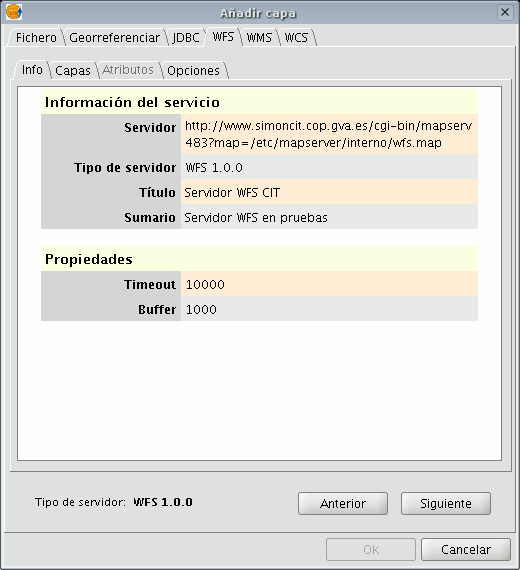
When you have accessed the service, a new group of tabs appears. The first tab (“Information”) shows all the information about the server and about the request that is to be sent. This information is updated as more layers are selected.
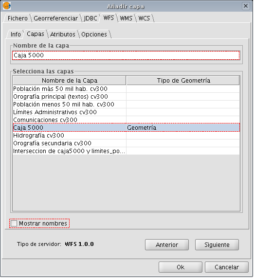
The “Layers” tab can be used to select the layer you wish to load. A two-column table appears in which the layer name and the geometry type are shown. As the geometry type is obtained by clicking on the layer (it needs to be obtained from the server), this column is completely blank at the start.
The “Show layer names” option shows the name of the layer as it is recognised by the server and not by its description, which is what appears in the table by default.
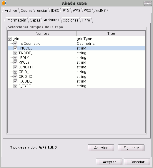
The “Attributes” tab allows the fields (or attributes) of the selected layer to be selected. When the layer is loaded, only the fields that have been selected are retrieved.
To select the attributes, enable the check box which appears to their left.
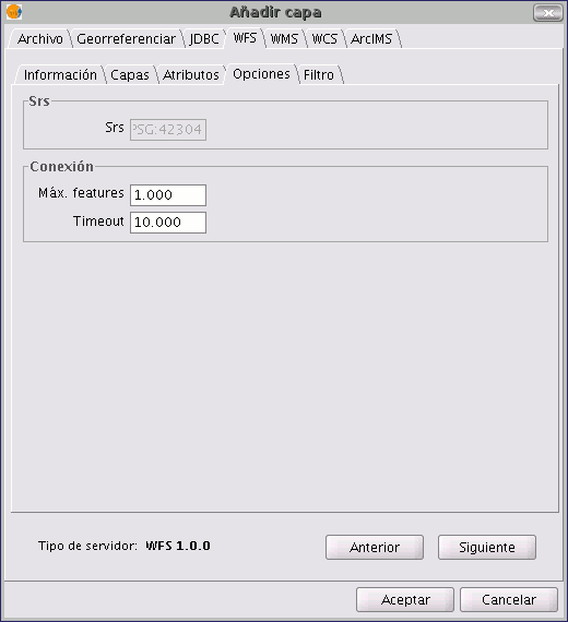
The "Options” tab shows information about user authentication and the connection. The “User” and “Password” fields are used in the WFS-T to be able to identify a user in the server so that writing operations can be carried out (not yet implemented).
The connection parameters are:
Number of features in the buffer, i.e. the maximum number of elements that can be downloaded.
Timeout. This is the length of time beyond which the connection is rejected as it is considered to be incorrect. If these parameters are very low, a correct request may not obtain a response.
The Spatial Reference System (SRS) is another important parameter. Although this cannot currently be changed, it is hoped that this will be possible in the future. In any case, gvSIG reprojects the loaded layer to the spatial system in the view.
You can use this tab to apply filters to your WFS layers. Click on the “Filters” tab in the window.
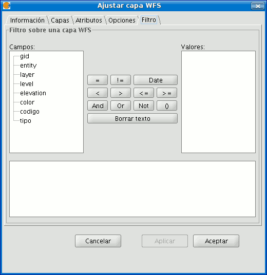
The “Fields” text box shows the layer’s attributes which can be used as a filter. Click on the selected field to see its values.
When the layer is loaded for the first time, the values in the column cannot be selected. However, if you have a filter sentence for the layer you can apply it in the filter text area and the filtered layer will be loaded directly.
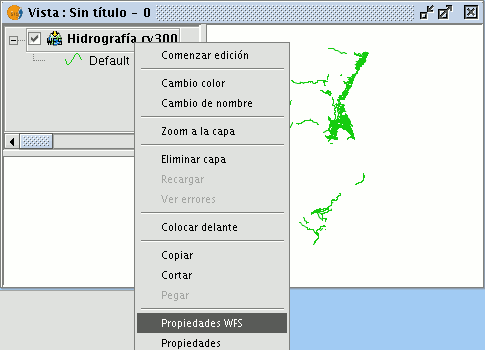
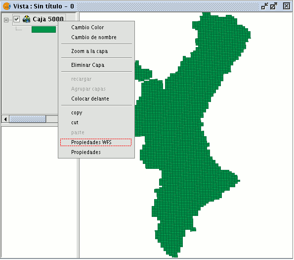
If you do not have a filter sentence, load the WFS layer into the ToC, then right click on the mouse and select the “WFS properties” option from the contextual menu.
To create the filter for the WFS layer, double click on the field you wish to use as a filter and it will appear in the bottom text area. Then click on the operator you wish to apply and finally select the value in the “Values” text area by double clicking on it.
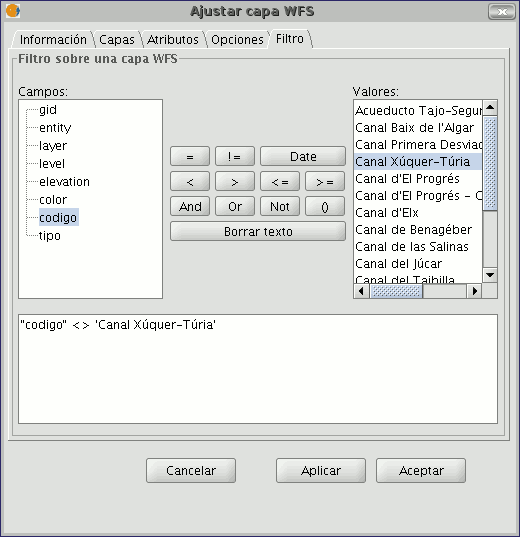
When you have created the required filter, click on “Ok” and it will be applied to the WFS layer.
When all the parameters have been configured, click on “Ok”. The layer will be loaded into a gvSIG view.
By right clicking on the layer, its contextual menu appears. If the “WFS Properties” option is selected, an option display opens (similar to the “Add layer” display). This can be used to select new attributes and other layers and change the layer’s properties.
In gvSIG 1.9 a new 'Area' tab was added which allows the user to filter the requested WFS layer geometries according to a bounding box. The user enters the coordinates of the required display area so as to optimize access to the data layers and to save time when viewing them.
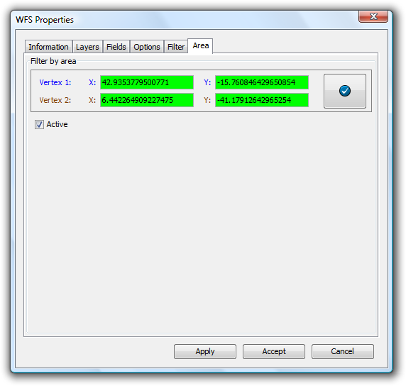
Loading a WFS layer - The Area tab
Adding a layer using vectorial ArcIMS protocol
In the proprietary software environment, ArcIMS (developed by Environmental Sciences Research Systems, ESRI) is probably the most widespread/popular widely used (Internet) cartographic server on the Internet thanks to the number of clients it supports (HTML, Java, ActiveX controls, ColdFusion...) and to its integration with other ESRI products. ArcIMS is currently one of the most important remote cartographic information providers. Although the protocol it uses does not comply with the Open Geospatial Consortium (because it was created long beforehand), the gvSIG team believes that offering support for ArcIMS is important.
The extension can access image services offered by an ArcIMS server. This means that, just like a WMS server, gvSIG can request a series of layers from a remote server and receive a view rendered by the server containing the requested layers in a specific coordinate system (reprojecting if necessary) and in specific dimensions. In addition to displaying geographic information, the extension allows you to request information about the layers for a particular point via the gvSIG standard information button.
ArcIMS is slightly different in its philosophy from WMS. In WMS, the request is normally made by independent layers whilst in ArcIMS the request is global.
The steps required to request a layer from an ArcIMS server and to request information for a particular point are listed below.
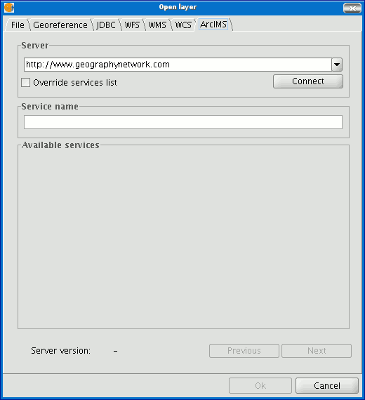
Our example uses the ESRI ArcIMS server. Its URL is http://www.geographynetwork.com. This is the address a web browser requires to access the HTML visual display unit.
Before loading a layer from this server, the datum WGS84 in geodesic coordinates (code 4326) has to be set up previously as the view’s spatial system.
If the extension is loaded correctly, a new ArcIMS data source will appear in the “Add layer” dialogue box.
Adding a new layer to the view
If the server has a standard configuration, simply indicate its address. gvSIG will try to find the servlet’s full address.1 If the servlet has a different path, you will have to write it into the dialogue box.
When the connection has successfully been made, the server version, its compilation number and a list of image and geometry services available are shown.
The service can be selected from the list or can be written in directly.
Finally, if the “Override service list” check box is enabled, gvSIG will delete any catalogue that has already been downloaded and will request them again from the server.
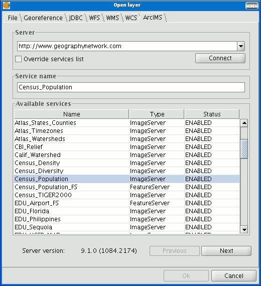
List of services available
The next step is to select the ImageServer type service required by double clicking or selecting it and clicking on "Next". The dialogue box changes and an interface with two tabs appears (fig. 3). The first tab shows the metainformation given by the server about the service’s geographic limits, the acronym of the language it has been written in, units of measurement, etc. It is a good idea to find out if a coordinate system has been defined in the service (using EPSG codes) as this can directly influence the requests made to the server, as Figure 3 shows.
N.B. If no coordinate system has been defined in the service, the extension will assume that it is the same coordinate system as the one we have defined for the view.
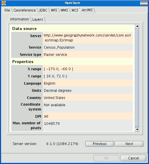
Figure 3: Metadata from the ArcIMS server
We can continue by clicking on "Next" or return to the previous dialogue by clicking on "Change service”.
The last dialogue box is the layer selection. We can define a name for the gvSIG layer or leave the default value (the service name) in this window. A box appears below with a list of the service layers in tree form. When the mouse is moved over the layers, information about these layers appears: extension, scale ranges, type of layer (raster or vector image) and if it is visible by default in the service (fig. 4).
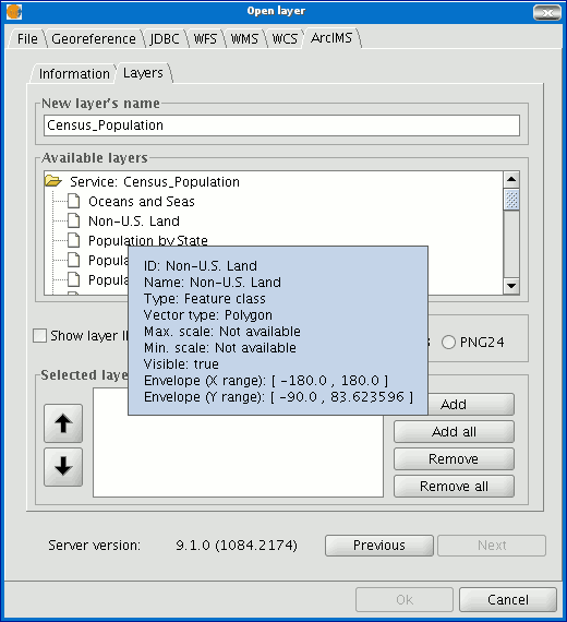
Figure 4: Metadata from a service layer
We can view each layer’s ID via the “Show layer ID” check box. This check box is useful when there are layers whose descriptor is repeated. Therefore, the only way to distinguish between them is via an ID, which will always be unique. A combo box is also available to select the image format we wish to use to download the images. We can choose JPG format if our service works with raster images or one of the other remaining formats if we want the service to have a transparent background.
N.B. The transparency in 24-bit PNG images is not correctly displayed in gvSIG 0.6. This type of files will be supported in gvSIG 1.0.
The box with the layers selected for the service appears below. If you wish, you can add just some of the service layers and also reorganise them. This makes the service view totally personalised.
N.B. The configuration cannot be accepted until a layer has been added.
N.B. Multiple selections of service layers can be made by using the Control and CAPS keys.
When the “Ok” button in the dialogue box is pressed, a new layer appears in the view (fig. 5). If no layer has been added previously, the extension of the ArcIMS layer is shown, as per the standard gvSIG procedure.
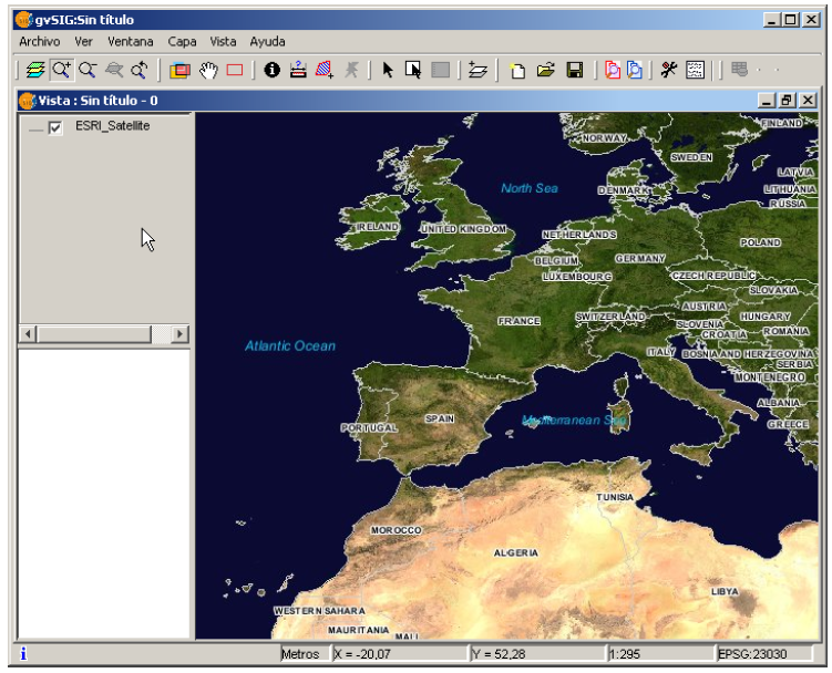
Figure 5: ArcIMS layer added to the gvSIG view.
It must be remembered that when the layer extension is shown, the layers that make up the chosen configuration may not appear and a blank or transparent image appears instead. If this occurs, use the scale control dialogue box (V. Information about scale limits section).
An ArcIMS server does not define the spatial reference systems it supports as opposed to the WMS specification. This means that a priori we do not have a list of EPSG codes that the map server can reproject. In short, ArcIMS can reproject to any coordinate system and leaves the responsibility of how the projections are used to the client.
Therefore, if our gvSIG view is defined in ED50 UTM zone 30 (EPSG:23030) and we request a global coverage service (stored for example in the geographic coordinates WGS84, which correspond to code 4326) the server will not be able to reproject the data correctly because we are using global coverage for a projection of a specific area of the Earth.
However, the procedure can be carried out in reverse. If we have a view in geographic coordinates (and thus global coverage), services defined in any coordinate system can be requested because the server will be able to transform the coordinates correctly.
In short, requests to the ArcIMS server must be made in the view's coordinate system and they cannot be requested in another coordinated system.
Moreover, as we mentioned above, if an ArcIMS server does not offer information about the coordinate system its data is in, the user will be responsible for setting up the correct coordinate system in the gvSIG view. Thus, if a user with a view in UTM adds a layer which is in geographic coordinates (even though the server does not show it), the service will be added correctly but will take the view to the geographic coordinates domain (in sexagesimal degrees).
An additional effect is that if the view uses different units of measurement from the server, the scale will not be shown correctly.
The layers requested from the server can be modified via a dialogue box, which can be accessed from the layer’s contextual menu (fig. 6) just like the WMS layers. This dialogue box is similar to the box used to load the layer, apart from the fact that the service cannot be changed.
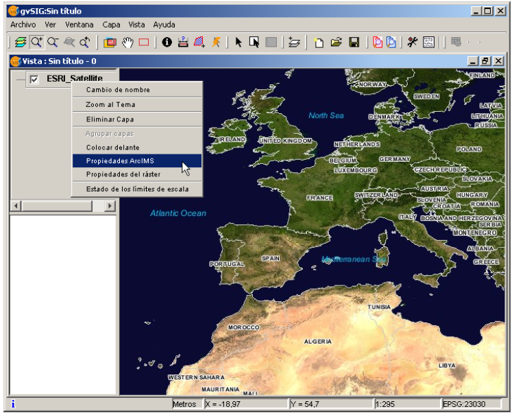
Figure 6: Properties of the ArcIMS layer
The extension allows us to consult the layers' scale limits which make up the requested service via a dialogue box which can be maintained in the view during the session (fig. 7). This window shows the layers on the vertical axis and the different scale denominators on the horizontal axis via a logarithmic scale. This box is small on screen but can be enlarged to improve the difference between the scales.
The vector layers, raster layers and the layers that can be seen on the current scale (marked with a vertical line) in a darker colour and the layers we cannot see above or below the current scale are differentiated by different coloured bars (described in the window legend).
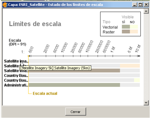
Figure 7: Scale limits status
Attribute information requests about the elements for a particular point is one of gvSIG’s standard tools. Its functionality is also supported by the extension.
The WMS specification allows information about several layers to be requested from the server in one single query. This is different in ArcIMS. We need to make one server request per layer required.
This means that no requests for unloaded layers or unseen layers that are not visible on the current scale or layers whose extension is outside the view will be made. Even if all these layers are filtered, the information request usually takes longer than is desirable because of this intrinsic feature of ArcIMS.
When all the request responses have been recovered, the standard gvSIG attribute information dialogue appears with each of the layers (LAYER) which return information as a tree. If we click on a layer, its name and ID appear on the right (fig. 8).
Under this node, if we are talking about a vector layer, all the records or geometric elements the server has responded to appear, and give each one their corresponding attributes (FIELDS).
If it is a raster layer, such as an orthoimage or a digital terrain model, it returns the values for each of the bands (BAND) in the requested pixel colour, instead of records.
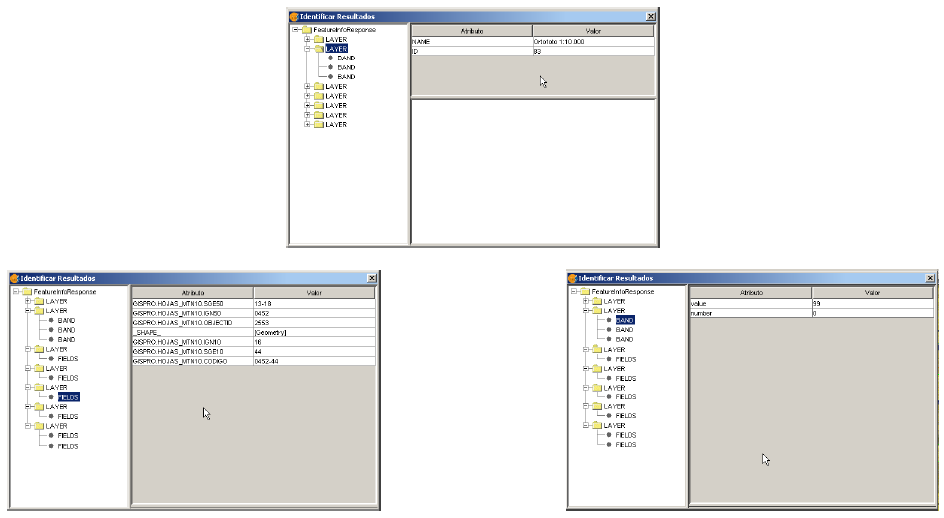
Figure 8: Displaying attribute information
The extension allows access to both ArcIMS image services and geometry services (Feature Services). This means that a server can be connected to and geometric entities (points, lines and polygons) and their attributes obtained. This is not dissimilar to WFS service access.
However, the variety of existing geometry services is much lower than the variety in the image server. There are two main reasons for this. On one hand, providing the public with vector cartography implies security problems because many bodies only want to offer the general public views and images. The vector data becomes either an internal product or must be paid for. On the other hand, this type of services generate much more traffic on the network and in the case of basic information servers could become a problem.
Loading a geometry layer is practically the same procedure as loading the image server as mentioned above (Accessing the service section and the following sections). In this case, the number of layers to be selected must be taken into account. If we wish to download all the layers offered by the service the response time will be very high.
The only difference between loading an image layer is that in this case we can choose whether we wish the layers to be downloaded as a group via a check box. This is useful for processing the vector layers as one layer when it needs to be moved and activated in the table of contents.
Unlike the image service, in which all the service’s layers appear as one unique layer in the gvSIG view, in this case each layer is downloaded separately and appears in the view grouped under the name defined in the connection dialogue.
Cartography symbols are configured in the server in one AXL extension file for both geometry and image services. We can divide symbol definition into two parts. On one hand, we can talk about the definition of the symbols themselves, i.e. how a geometric element, such as a line or polygon, should be presented. On the other hand, we can talk about the distribution of these symbols according to the cartographic display scale or to a specific theme attribute.
In ArcIMS terminology symbols are different from legends (SYMBOLS and RENDERERS).
There are various types of symbols: raster fill symbols, gradient fill symbols, simple line symbol, etc. The extension adapts the majority of the symbols generated by ArcIMS. Table 1 shows the ArcIMS symbols and indicates whether they are supported by gvSIG.
| Label | Description | Supported |
|---|---|---|
| CALLOUTMARKERSYMBOL | Balloon-type label | NO |
| CHARTSYMBOL | Pie chart symbol | NO |
| GRADIENTFILLSYMBOL | Fill in with gradient | NO |
| RASTERFILLSYMBOL | Fill with raster pattern | YES |
| RASTERMARKERSYMBOL | Point symbol using pictogram | YES |
| RASTERSHIELDSYMBOL | Customised point symbol for US roads | NO |
| SIMPLELINESYMBOL | Simple line | YES |
| SIMPLEMARKERSYMBOL | Point | YES |
| SIMPLEPOLYGONSYMBOL | Polygon | YES |
| SHIELDSYMBOL | Point symbol for US roads | NO |
| TEXTMARKERSYMBOL | Static text symbol | NO |
| TEXTSYMBOL | Static text symbol | YES |
| TRUETYPEMARKERSYMBOL | Symbol using TrueType font character | NO |
Table 1: ArcXML symbol definition labels
In general, the most common symbols have been successfully “transferred”. Some of the symbols cannot be obtained directly from gvSIG (at least in the current version), such as the raster fill symbol or they need to be “adjusted” such as the different types of lines. This means that a raster fill symbol is not a symbol that can be defined by the gvSIG user interface, but it can be defined by programming.
gvSIG supports the most common types of legends: unique value and range and value themes as well as the scale-range control over the whole layer. ArcIMS goes much further in its configuration. It can generate much more complicated legends in which symbols can be grouped together, scale-range controls can be established for labels and symbols and different labelling based on an attribute can be shown (as though it were a value theme for labelling).
This group of legends can generate very complex symbols for a layer in the end. The current implementation status of the gvSIG symbols needs to be simplified to reach a compromise to recover the symbols that best represent the layer as a whole.
| Label | Description |
|---|---|
| GROUPRENDERER | Legend which groups others together |
| SCALEDEPENDENTRENDERER | Scale dependent legend |
| SIMPLELABELRENDERER | Labelling layer legend |
| SIMPLERENDERER | Unique value layer legend |
| VALUEMAPRENDERER | Value and range themes |
| VALUEMAPLABELRENDERER | Labelling themes |
Table 2: ArcXML legend definition labels
When a GROUPRENDERER is found, the symbol ArcIMS draws first is always chosen. Thus, in the case of the typical motorway symbol for which a thick red line is drawn and a thinner yellow line is drawn over it, gvSIG will only show the red line with its specific thickness.
If a scale dependent legend is discovered during a symbol analysis, this is always chosen. If more than one is discovered, the one with the greatest detail is chosen. For example, in ArcIMS we can have a layer with simple road symbols (only main roads are drawn) on a 1:250000 scale and based on this a different theme is shown with all types of roads (paths, tracks, roads, etc.). In this case, gvSIG will show this last theme as it is the most detailed.
If a labelling legend is discovered during a symbol analysis, it will be saved in a different place and will be assigned to the selected definitive legend. In the case of the VALUEMAPLABELRENDERER label, only the legend of the first processed value will be obtained as a label symbol. The rest will be rejected.
In short, it is obvious that the failure to adapt the legends for gvSIG is a simplification process in which different legend and symbol definitions must be rejected to obtain a legend which is similar to the original as far as possible. It is to be expected that the gvSIG symbol definition will improve considerably so that it can support a larger group of cases in the future.
Working with the layer is similar to any other vector layer, as long as we remember that access times may be relatively high. The layer attribute table can be consulted, in which case the records will be downloaded successively as we display them.
If we wish to change the table symbols to show a unique value or range theme we must wait as gvSIG requests the complete table for these operations. On the other hand, the downloading of attributes is only carried out once per layer and session and therefore, this wait only occurs in the first operation.
In general, if our ArcIMS server is in an Intranet, it will be relatively fast to handle, but if we wish to access remote services we may be faced with considerable response times.
The main feature to bear in mind when working with an ArcIMS vector layer is that the geometries available at any given time are only the ones displayed. This is because we can connect to huge layers but only the visible geometries are downloaded. As far as gvSIG is concerned, the geometries shown on the screen are the only ones available and thus, if we export the view to a shapefile for example, are only a part of the layer.
Finally, we need to remember that to speed up the geometry downloads they are simplified to the viewing scale in use at any given time. This drastically reduces the amount of information downloaded as only the geometries that can actually be "drawn" are displayed in the view.
Loading a geometry layer is practically the same procedure as loading the image server as mentioned above (Accessing the service section and the following sections). In this case, the number of layers to be selected must be taken into account. If we wish to download all the layers offered by the service the response time will be very high.
Unlike the image service, in which all the service’s layers appear as one unique layer in the gvSIG view, in this case each layer is downloaded separately and appear in the view grouped under the name defined in the connection dialogue.
After a few seconds the layers appear individually but are grouped under a layer with the name we have defined for it.
The layer symbols are established at random. A pending feature is to recover the service symbols and configure them by default so that gvSIG can display the cartography as similarly as possible to how it was established by the service administrator.
Raster
Adding a layer from a disk file
Click on the "Add" button
The "Add” dialogue window allows you to move around the file system to select the layer to be loaded. Remember that only the files of the type selected will be shown. To indicate the type of file to be loaded, select a file from the “Files of type” pull down menu.
If several layers are loaded at the same time, the order in which the themes will be added to the view can be specified with the "Up" and "Down" buttons in the “Add layer" dialogue.
Adding a layer usins WMS protocol
Part of the gvSIG philosophy in its creation included the implementation of open standards for access to spatial data. Thus, gvSIG includes a WMS client which complies with the current OGC (Open Geospatial Consortium, http://www.opengeospatial.org) standard.
Go to the "Add layer" window and then select the WMS tab.
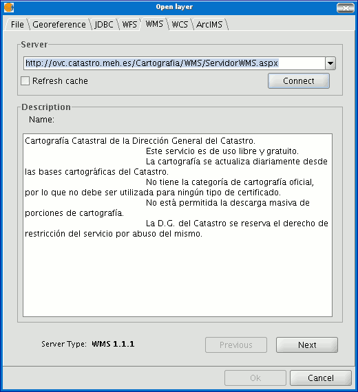
- The pull-down menu shows a list of WMS servers (you can add a different server if you don’t find the one you want).
- Click on “Connect”.
- and 4. When the connection is made, a welcome message from the server appears, if this has been configured. If no welcome message appears, you can check whether you have successfully connected to the server if the “Next” button is enabled.
- The WMS version number that the connection has been made to is shown at the bottom of the box.
Click on “Next” to start configuring the new WMS layer.
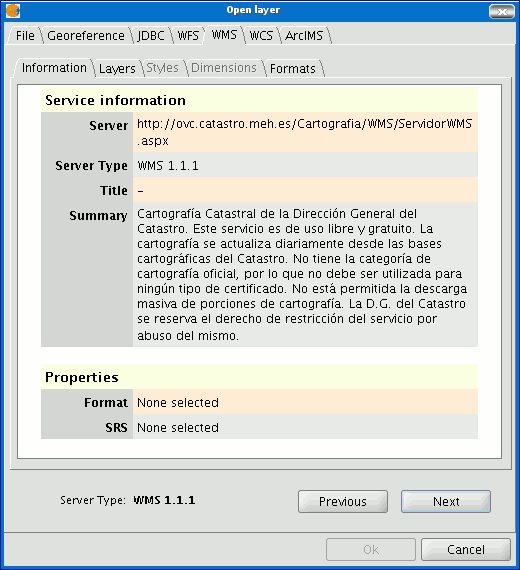
When you have accessed the service, a new group of tabs appears.
The first tab in the adding a WMS layer wizard is the information tab. It summarises the current configuration of the WMS request (service information, formats, spatial systems, layers which make up the request, etc.). This tab is updated as the properties of its request are changed, added or deleted.
The wizard’s “Layers” tab shows the WMS server’s table of contents.
Select the layers you wish to add to your gvSIG view and click on “Add”. If you wish, you can choose a name for the layer in the “Layer name” field.
N.B. Several layers can be selected at the same time by holding down the “Control” key and left clicking on the mouse.
N.B. To obtain a layer description move the cursor over a layer and wait a few seconds. The information the server has about these layers is shown.
The “Styles” tab allows you to choose a display view for the selected layers. However, this is an optional property and the tab may be disabled because the server does not define styles for the selected layers.
The “Dimensions” tab helps to configure the value for the WMS layer dimensions. However, the dimensions property (like the styles property) is optional and may be disabled if the server does not specify dimensions for the selected layers.
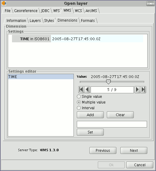
No dimension is configured by default. To add a dimension, select one from the “Settings editor” area in the list of dimensions. The controls in the bottom right-hand corner of the tab are enabled. Use the slider control to move through the list of values the server has defined for the selected dimension (for example “TIME” refers to the dates the different images were taken). You can move back to the beginning, one step back, one step forward or move to the end of the list using the navigation buttons which are located below the slider control. If you know the position of the value you require, you can simply write it in the text field and it will move automatically to this value.
Click on “Add” so that you can write the selected value in the text field and request it from the server.
gvSIG allows you to choose between:
Single value: Only one value is selected
Multiple value: The values will be added to the list in the order they are selected in
Interval: An initial value and then an end value are selected
When the expression for your dimension is complete, click on “Set” and the expression will appear in the information panel.
N.B. Although each layer can define its own dimensions, only one choice of value is permitted (single, multiple or interval) for each variable (e.g. for the TIME variable a different image date value cannot be chosen in each layer).
N.B. The server may come into conflict with the layer combination and the variable value you have chosen. Some of the layers you have chosen may not support your selected value. If this occurs, a server error message will appear.
N.B. You can personalise the expression in the text field. The dialogue box controls are only designed to make it easier to edit dimension expressions. If you wish you can edit the text field at any time.
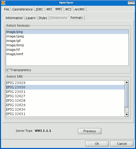
The “Formats” tab allows you to choose the image format the request will be made with, specify if you wish the server to hand in the image with a transparency (to superimpose the layer onto other layers the gvSIG view already contains) and also the spatial reference system (SRS) you require.
As soon as the configuration is sufficient to place the request, the “Ok” button is enabled. If you click on this button, the new WMS layer will be added to the gvSIG view.
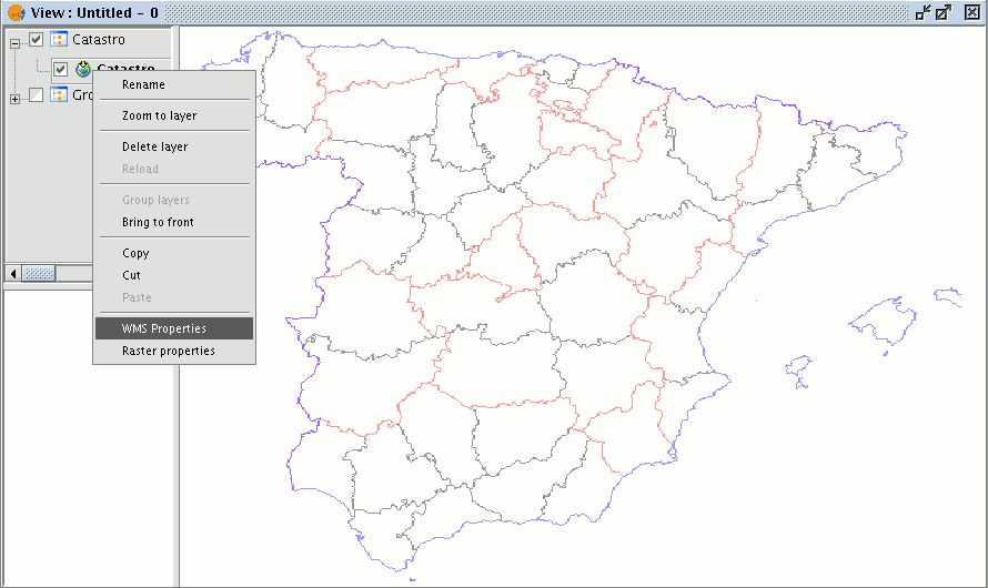
Once the layer has been added its properties can be modified. To do so, go to the Table of contents in your gvSIG view and right click on the WMS layer you wish to modify. The contextual menu of layer operations appears. Select “WMS Properties”. The “Config WMS layer” dialogue window appears. This is similar to the wizard for creating the WMS layer and can be used to modify its configurations.
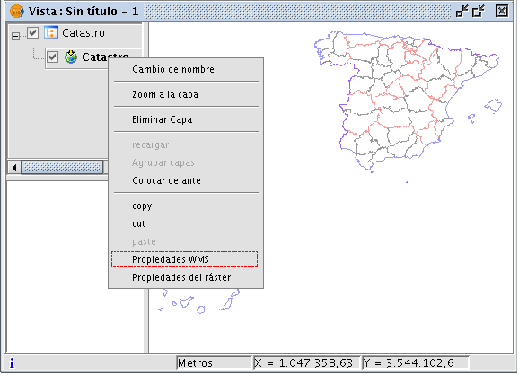
Adding a layer using WCS protocol
The WCS (Web Coverage Service) is another of the OGC standards supported by gvSIG. The WCS is a coverage server. It is different from WMS as this standard defines a map as a representation of geographic information in the shape of a digital image file which can be shown on a computer screen. The map does not include its own data but WCS, however, does provide its own data, which can subsequently be analysed. WCS therefore allows raster data to be analysed just as WFS allows vector data to be analysed.
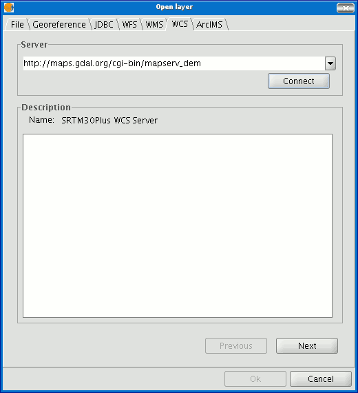
- The pull-down menu shows a list of WCS servers (you can add a different server if you don’t find the one you want).
- Click on “Connect”. gvSIG connects to the server.
- and 4. When the connection is made, a welcome message from the server appears, if this has been configured. If no welcome message appears, you can check whether you have successfully connected to the server if the “Next” button is enabled.
Click on “Next” to start configuring the new WCS layer.
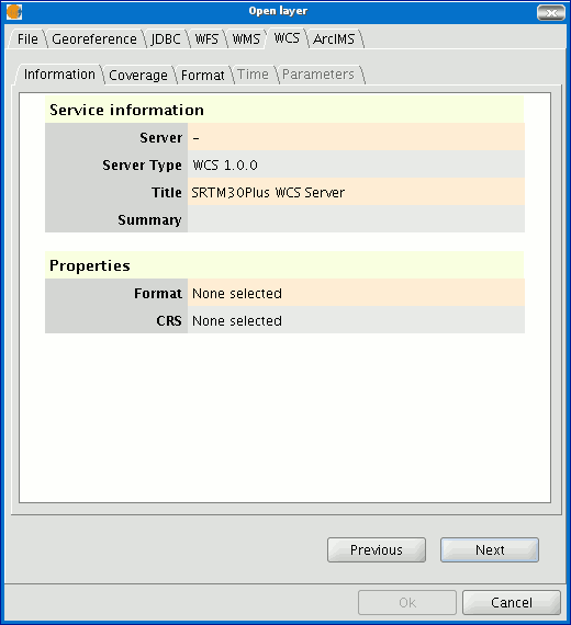
When you have accessed the service, a new group of tabs appears.
The first tab in the adding a WCS layer wizard is the information tab. It summarises the current configuration of the WCS request (service information, formats, spatial systems, layers which make up the request, etc.). This tab is updated as the properties of its request are changed, added or deleted.
Select the coverage you wish to add to your gvSIG view. If you wish, you can choose a name for your layer in the “Coverage name” field.
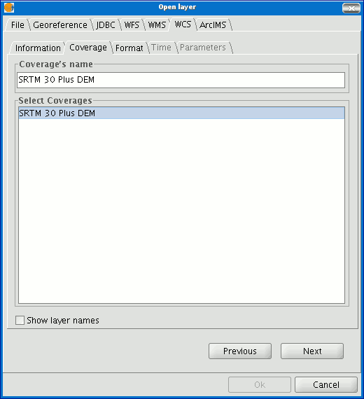
You can choose the image format you wish to use to make the request and reference system (SRS) in the “Format” tab.
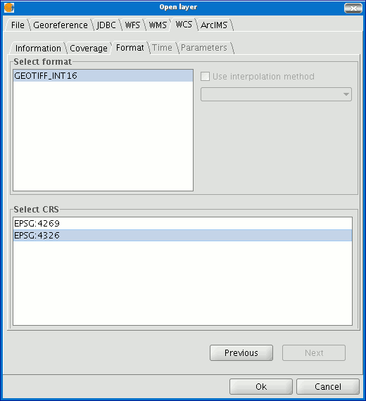
N.B. Tabs such as “Time” and “Parameters” are disabled in this case. Configuring these variables depends on the server chosen and the type of data it has access to.
As soon as the configuration is sufficient to place the request, the “Ok” button is enabled. If you click on this button, the new WCS layer will be added to the gvSIG view.
Once the layer has been added its properties can be modified. To do so, go to the Table of contents in your gvSIG view and right click on the WCS layer you wish to modify. The contextual menu of layer operations appears. Select “WCS Properties”.
The “Config WCS layer” dialogue window appears. This is similar to the wizard for creating the WMS layer and can be used to modify your configurations.
Adding orthophotos using the ECWP protocol
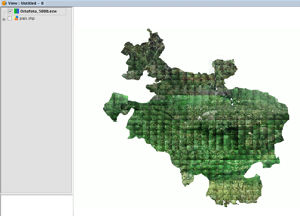
If you wish to add an orthophoto to gvSIG using the ECWP protocol, first open a view and click on the “Add layer” button.

Click on the “Add” button in the dialogue box. A file browser window appears.
Choose the “gvSIG Image Driver” option from the “Files of type” pull-down menu.
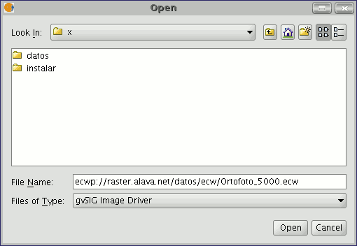
Write the URL of the file you wish to load as follows in “File name”:
ecwp://server address/path of the file you wish to add.
For example:
ecwp://raster.alava.net/datos/ecw/Ortofoto_5000.ecw
ecwp://earthetc.com/images/geodetic/world/MOD09A1.interpol.cyl.retouched.topo.bathymetry.ecw
When you have input the data, click on “Open”.
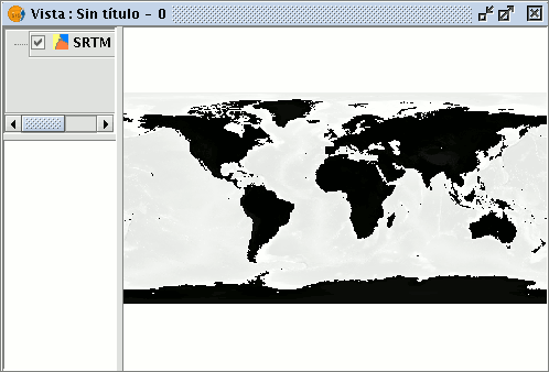
The orthophoto will be added to the layer list.
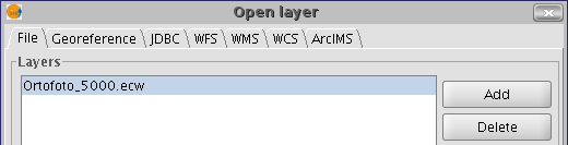
Select the new added layer and click on “Ok”.
The image will be added to the view.
Adding a layer using raster ArcIMS protocol
In the proprietary software environment, ArcIMS (developed by Environmental Sciences Research Systems, ESRI) is probably the most widespread/popular widely used (Internet) cartographic server on the Internet thanks to the number of clients it supports (HTML, Java, ActiveX controls, ColdFusion...) and to its integration with other ESRI products. ArcIMS is currently one of the most important remote cartographic information providers. Although the protocol it uses does not comply with the Open Geospatial Consortium (because it was created long beforehand), the gvSIG team believes that offering support for ArcIMS is important.
The extension can access image services offered by an ArcIMS server. This means that, just like a WMS server, gvSIG can request a series of layers from a remote server and receive a view rendered by the server containing the requested layers in a specific coordinate system (reprojecting if necessary) and in specific dimensions. In addition to displaying geographic information, the extension allows you to request information about the layers for a particular point via the gvSIG standard information button.
ArcIMS is slightly different in its philosophy from WMS. In WMS, the request is normally made by independent layers whilst in ArcIMS the request is global.
The steps required to request a layer from an ArcIMS server and to request information for a particular point are listed below.
Our example uses the ESRI ArcIMS server. Its URL is http://www.geographynetwork.com. This is the address a web browser requires to access the HTML visual display unit.
Before loading a layer from this server, the datum WGS84 in geodesic coordinates (code 4326) has to be set up previously as the view’s spatial system.
If the extension is loaded correctly, a new ArcIMS data source will appear in the “Add layer” dialogue box.
Adding a new layer to the view
If the server has a standard configuration, simply indicate its address. gvSIG will try to find the servlet’s full address.1 If the servlet has a different path, you will have to write it into the dialogue box.
When the connection has successfully been made, the server version, its compilation number and a list of image and geometry services available are shown.
The service can be selected from the list or can be written in directly.
Finally, if the “Override service list” check box is enabled, gvSIG will delete any catalogue that has already been downloaded and will request them again from the server.
List of services available
The next step is to select the ImageServer type service required by double clicking or selecting it and clicking on "Next". The dialogue box changes and an interface with two tabs appears (fig. 3). The first tab shows the metainformation given by the server about the service’s geographic limits, the acronym of the language it has been written in, units of measurement, etc. It is a good idea to find out if a coordinate system has been defined in the service (using EPSG codes) as this can directly influence the requests made to the server, as Figure 3 shows.
N.B. If no coordinate system has been defined in the service, the extension will assume that it is the same coordinate system as the one we have defined for the view.
Figure 3: Metadata from the ArcIMS server
We can continue by clicking on "Next" or return to the previous dialogue by clicking on "Change service”.
The last dialogue box is the layer selection. We can define a name for the gvSIG layer or leave the default value (the service name) in this window. A box appears below with a list of the service layers in tree form. When the mouse is moved over the layers, information about these layers appears: extension, scale ranges, type of layer (raster or vector image) and if it is visible by default in the service (fig. 4).
Figure 4: Metadata from a service layer
We can view each layer’s ID via the “Show layer ID” check box. This check box is useful when there are layers whose descriptor is repeated. Therefore, the only way to distinguish between them is via an ID, which will always be unique. A combo box is also available to select the image format we wish to use to download the images. We can choose JPG format if our service works with raster images or one of the other remaining formats if we want the service to have a transparent background.
N.B. The transparency in 24-bit PNG images is not correctly displayed in gvSIG 0.6. This type of files will be supported in gvSIG 1.0.
The box with the layers selected for the service appears below. If you wish, you can add just some of the service layers and also reorganise them. This makes the service view totally personalised.
N.B. The configuration cannot be accepted until a layer has been added.
N.B. Multiple selections of service layers can be made by using the Control and CAPS keys.
When the “Ok” button in the dialogue box is pressed, a new layer appears in the view (fig. 5). If no layer has been added previously, the extension of the ArcIMS layer is shown, as per the standard gvSIG procedure.
Figure 5: ArcIMS layer added to the gvSIG view.
It must be remembered that when the layer extension is shown, the layers that make up the chosen configuration may not appear and a blank or transparent image appears instead. If this occurs, use the scale control dialogue box (V. Information about scale limits section).
An ArcIMS server does not define the spatial reference systems it supports as opposed to the WMS specification. This means that a priori we do not have a list of EPSG codes that the map server can reproject. In short, ArcIMS can reproject to any coordinate system and leaves the responsibility of how the projections are used to the client.
Therefore, if our gvSIG view is defined in ED50 UTM zone 30 (EPSG:23030) and we request a global coverage service (stored for example in the geographic coordinates WGS84, which correspond to code 4326) the server will not be able to reproject the data correctly because we are using global coverage for a projection of a specific area of the Earth.
However, the procedure can be carried out in reverse. If we have a view in geographic coordinates (and thus global coverage), services defined in any coordinate system can be requested because the server will be able to transform the coordinates correctly.
In short, requests to the ArcIMS server must be made in the view's coordinate system and they cannot be requested in another coordinated system.
Moreover, as we mentioned above, if an ArcIMS server does not offer information about the coordinate system its data is in, the user will be responsible for setting up the correct coordinate system in the gvSIG view. Thus, if a user with a view in UTM adds a layer which is in geographic coordinates (even though the server does not show it), the service will be added correctly but will take the view to the geographic coordinates domain (in sexagesimal degrees).
An additional effect is that if the view uses different units of measurement from the server, the scale will not be shown correctly.
The layers requested from the server can be modified via a dialogue box, which can be accessed from the layer’s contextual menu (fig. 6) just like the WMS layers. This dialogue box is similar to the box used to load the layer, apart from the fact that the service cannot be changed.
Figure 6: Properties of the ArcIMS layer
The extension allows us to consult the layers' scale limits which make up the requested service via a dialogue box which can be maintained in the view during the session (fig. 7). This window shows the layers on the vertical axis and the different scale denominators on the horizontal axis via a logarithmic scale. This box is small on screen but can be enlarged to improve the difference between the scales.
The vector layers, raster layers and the layers that can be seen on the current scale (marked with a vertical line) in a darker colour and the layers we cannot see above or below the current scale are differentiated by different coloured bars (described in the window legend).
Figure 7: Scale limits status
Attribute information requests about the elements for a particular point is one of gvSIG’s standard tools. Its functionality is also supported by the extension.
The WMS specification allows information about several layers to be requested from the server in one single query. This is different in ArcIMS. We need to make one server request per layer required.
This means that no requests for unloaded layers or unseen layers that are not visible on the current scale or layers whose extension is outside the view will be made. Even if all these layers are filtered, the information request usually takes longer than is desirable because of this intrinsic feature of ArcIMS.
When all the request responses have been recovered, the standard gvSIG attribute information dialogue appears with each of the layers (LAYER) which return information as a tree. If we click on a layer, its name and ID appear on the right (fig. 8).
Under this node, if we are talking about a vector layer, all the records or geometric elements the server has responded to appear, and give each one their corresponding attributes (FIELDS).
If it is a raster layer, such as an orthoimage or a digital terrain model, it returns the values for each of the bands (BAND) in the requested pixel colour, instead of records.
Figure 8: Displaying attribute information
The extension allows access to both ArcIMS image services and geometry services (Feature Services). This means that a server can be connected to and geometric entities (points, lines and polygons) and their attributes obtained. This is not dissimilar to WFS service access.
However, the variety of existing geometry services is much lower than the variety in the image server. There are two main reasons for this. On one hand, providing the public with vector cartography implies security problems because many bodies only want to offer the general public views and images. The vector data becomes either an internal product or must be paid for. On the other hand, this type of services generate much more traffic on the network and in the case of basic information servers could become a problem.
Loading a geometry layer is practically the same procedure as loading the image server as mentioned above (Accessing the service section and the following sections). In this case, the number of layers to be selected must be taken into account. If we wish to download all the layers offered by the service the response time will be very high.
The only difference between loading an image layer is that in this case we can choose whether we wish the layers to be downloaded as a group via a check box. This is useful for processing the vector layers as one layer when it needs to be moved and activated in the table of contents.
Unlike the image service, in which all the service’s layers appear as one unique layer in the gvSIG view, in this case each layer is downloaded separately and appears in the view grouped under the name defined in the connection dialogue.
Cartography symbols are configured in the server in one AXL extension file for both geometry and image services. We can divide symbol definition into two parts. On one hand, we can talk about the definition of the symbols themselves, i.e. how a geometric element, such as a line or polygon, should be presented. On the other hand, we can talk about the distribution of these symbols according to the cartographic display scale or to a specific theme attribute.
In ArcIMS terminology symbols are different from legends (SYMBOLS and RENDERERS).
There are various types of symbols: raster fill symbols, gradient fill symbols, simple line symbol, etc. The extension adapts the majority of the symbols generated by ArcIMS. Table 1 shows the ArcIMS symbols and indicates whether they are supported by gvSIG.
| Label | Description | Supported |
|---|---|---|
| CALLOUTMARKERSYMBOL | Balloon-type label | NO |
| CHARTSYMBOL | Pie chart symbol | NO |
| GRADIENTFILLSYMBOL | Fill in with gradient | NO |
| RASTERFILLSYMBOL | Fill with raster pattern | YES |
| RASTERMARKERSYMBOL | Point symbol using pictogram | YES |
| RASTERSHIELDSYMBOL | Customised point symbol for US roads | NO |
| SIMPLELINESYMBOL | Simple line | YES |
| SIMPLEMARKERSYMBOL | Point | YES |
| SIMPLEPOLYGONSYMBOL | Polygon | YES |
| SHIELDSYMBOL | Point symbol for US roads | NO |
| TEXTMARKERSYMBOL | Static text symbol | NO |
| TEXTSYMBOL | Static text symbol | YES |
| TRUETYPEMARKERSYMBOL | Symbol using TrueType font character | NO |
Table 1: ArcXML symbol definition labels
In general, the most common symbols have been successfully “transferred”. Some of the symbols cannot be obtained directly from gvSIG (at least in the current version), such as the raster fill symbol or they need to be “adjusted” such as the different types of lines. This means that a raster fill symbol is not a symbol that can be defined by the gvSIG user interface, but it can be defined by programming.
gvSIG supports the most common types of legends: unique value and range and value themes as well as the scale-range control over the whole layer. ArcIMS goes much further in its configuration. It can generate much more complicated legends in which symbols can be grouped together, scale-range controls can be established for labels and symbols and different labelling based on an attribute can be shown (as though it were a value theme for labelling).
This group of legends can generate very complex symbols for a layer in the end. The current implementation status of the gvSIG symbols needs to be simplified to reach a compromise to recover the symbols that best represent the layer as a whole.
| Label | Description |
|---|---|
| GROUPRENDERER | Legend which groups others together |
| SCALEDEPENDENTRENDERER | Scale dependent legend |
| SIMPLELABELRENDERER | Labelling layer legend |
| SIMPLERENDERER | Unique value layer legend |
| VALUEMAPRENDERER | Value and range themes |
| VALUEMAPLABELRENDERER | Labelling themes |
Table 2: ArcXML legend definition labels
When a GROUPRENDERER is found, the symbol ArcIMS draws first is always chosen. Thus, in the case of the typical motorway symbol for which a thick red line is drawn and a thinner yellow line is drawn over it, gvSIG will only show the red line with its specific thickness.
If a scale dependent legend is discovered during a symbol analysis, this is always chosen. If more than one is discovered, the one with the greatest detail is chosen. For example, in ArcIMS we can have a layer with simple road symbols (only main roads are drawn) on a 1:250000 scale and based on this a different theme is shown with all types of roads (paths, tracks, roads, etc.). In this case, gvSIG will show this last theme as it is the most detailed.
If a labelling legend is discovered during a symbol analysis, it will be saved in a different place and will be assigned to the selected definitive legend. In the case of the VALUEMAPLABELRENDERER label, only the legend of the first processed value will be obtained as a label symbol. The rest will be rejected.
In short, it is obvious that the failure to adapt the legends for gvSIG is a simplification process in which different legend and symbol definitions must be rejected to obtain a legend which is similar to the original as far as possible. It is to be expected that the gvSIG symbol definition will improve considerably so that it can support a larger group of cases in the future.
Working with the layer is similar to any other vector layer, as long as we remember that access times may be relatively high. The layer attribute table can be consulted, in which case the records will be downloaded successively as we display them.
If we wish to change the table symbols to show a unique value or range theme we must wait as gvSIG requests the complete table for these operations. On the other hand, the downloading of attributes is only carried out once per layer and session and therefore, this wait only occurs in the first operation.
In general, if our ArcIMS server is in an Intranet, it will be relatively fast to handle, but if we wish to access remote services we may be faced with considerable response times.
The main feature to bear in mind when working with an ArcIMS vector layer is that the geometries available at any given time are only the ones displayed. This is because we can connect to huge layers but only the visible geometries are downloaded. As far as gvSIG is concerned, the geometries shown on the screen are the only ones available and thus, if we export the view to a shapefile for example, are only a part of the layer.
Finally, we need to remember that to speed up the geometry downloads they are simplified to the viewing scale in use at any given time. This drastically reduces the amount of information downloaded as only the geometries that can actually be "drawn" are displayed in the view.
Loading a geometry layer is practically the same procedure as loading the image server as mentioned above (Accessing the service section and the following sections). In this case, the number of layers to be selected must be taken into account. If we wish to download all the layers offered by the service the response time will be very high.
Unlike the image service, in which all the service’s layers appear as one unique layer in the gvSIG view, in this case each layer is downloaded separately and appear in the view grouped under the name defined in the connection dialogue.
After a few seconds the layers appear individually but are grouped under a layer with the name we have defined for it.
The layer symbols are established at random. A pending feature is to recover the service symbols and configure them by default so that gvSIG can display the cartography as similarly as possible to how it was established by the service administrator.
Web Map Context
Web Map Context (WMC) is another OGC standard (http://www.opengeospatial.org) which can be added to the list of standards of this type supported by gvSIG.
It can reproduce a view made up of Web Map Services (WMS) layers on any GIS platform which supports WMC. If your project has a view which contains WMS layers, you can export these layers. The result is an XML file with a specific format and .cml extension which can be imported by another platform on which the view it describes can be reproduced.
Web Map Context (WMC) is another OGC standard (http://www.opengeospatial.org) which can be added to the list of standards of this type supported by gvSIG.
It can reproduce a view made up of Web Map Services (WMS) layers on any GIS platform which supports WMC.
If your project has a view which contains WMS layers, you can export these layers. The result is an XML file with a specific format and .cml extension which can be imported by another platform on which the view it describes can be reproduced.
Exporting a view to WMC
Exports to WMC are currently limited to WMS type layers, although it is hoped that its functions will extend to all layers that comply with OGC standards in the future.
To obtain a WMC file, open a view in gvSIG and add the WMS layers you require.
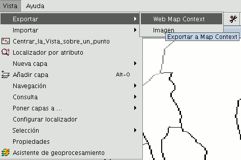
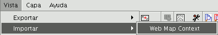
Then go to the “View” menu and select “Export” and then “Web Map Context”.
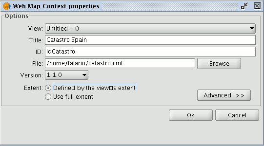
The following dialogue will be shown.
N.B.: If you cannot find the "Web Map Context" option in the "Export" option, your project does not contain any WMS layers.
Basic mode only shows the compulsory properties which cannot be taken for granted by the application.
View: This defines which view is going to be exported to the WMC. The view which is currently active is selected by default.
Title: This is the title of the view which will be shown when your .cml file is loaded at a later date. The current title of the view is used by default but this can be changed.
ID: This field is also compulsory and represents a file ID which must be unique.
File: You can search for the place you wish to save the .cml file in from the "Browse" button.
Version: Use this tool to specify the WMC version you wish to use.
The version 1.1.0 is selected by default as it is the most highly developed and the most recommended. However, several applications and geoportals are often limited to a specific version.
gvSIG currently supports Web Map Context in its versions 0.1.4, 1.0.0 and 1.1.0.
Extent: This defines the extension of the map to be exported.
Defined by the view’s extent. This option only exports what we can currently see in the view.
Use full extent. This extension is better to use the full WMS layers depending on how their respective servers define them.
If you click on the “Advanced” button, the advanced configuration dialogue will drop down. This allows you to define more properties to obtain a complete WMC.
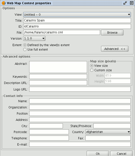
Abstract: This contains a summary of the view defined by WMC.
Keywords: This list of words allows you to classify and “metadata” the WMC.
URL description: If you have a web site which refers to this WMC, write its link here.
URL logo: If you have an image associated with this WMC, write its link here.
Map size (pixels): This defines the pixel size that the WMC-defined view will have. The current gvSIG view size is used by default but you can customise the size if you wish.
Contact info: Information that allows third parties to contact the WMC author.
Importing Web Map Context allows you to use gvSIG to open views with WMS layers which have been created with other platforms or with another gvSIG.
Use the "View” menu and select “Import” and then “Web Map Context”.
The WMC file selection dialogue opens.
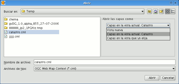
Choose the WMC file you wish to import. On the right, you can specify how you wish to view the layers.
New view: This adds a new view to the current project and loads the WMC as specified in the file.
Layers in the active (current) view: This option only appears if the active gvSIG window is a view. It allows you to quickly add the layers to the current view.
Layers in other view: This adds the layers defined by the WMC in the chosen view. In this option, a list of views appears to select the view that will contain the new layers.
Click on the “Open” button to import the file based on your preferences.
Alfanumeric
File
introduction
Tables are documents which contain alphanumeric information. Tables are made up of rows or records (which represent each of the elements in the data base) and columns or fields (which define the different attributes of each element).
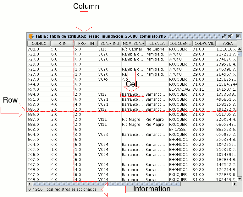
Row or record: Used to represent the different elements in the table.
Column or field: The types of attributes which define each element.
Cell: A cell is the intersection of a record and a field. A cell is the minimum working element and may contain information.
Record information: This provides information about the total number of elements (records) contained in the table.
All the vector information layers have their own “Table of attributes”. Each graphic element in a particular layer has its corresponding record in the “Table of attributes”.
To select elements in the table, left click on them. Use the “Control” and “Shift” (CAPS) keys to select more than one record.
Adding a table
You can load a table in gvSIG in two ways:
- From the “Project manager”
- From the “View”
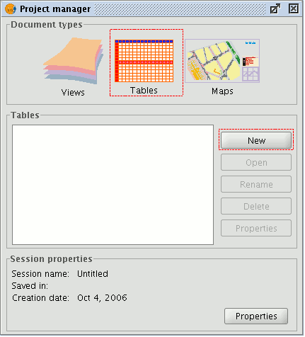
Select “Tables” as the document type from the “Project manager” and click on “New”. A dialogue box will open in which you can add the table.
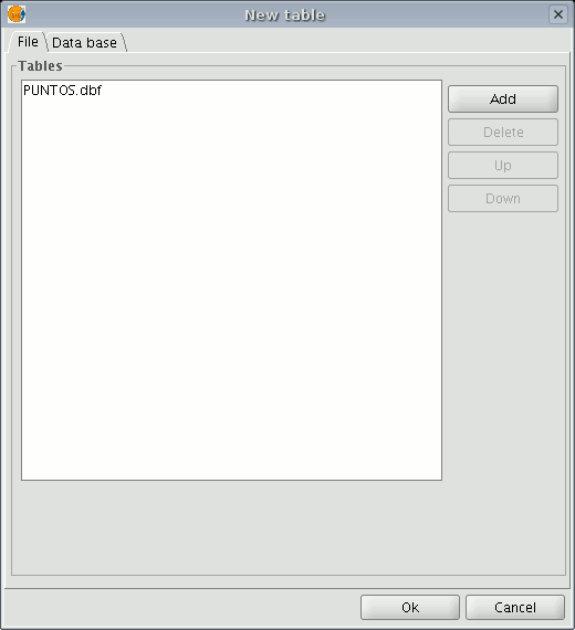
When you click on the “Add” button, a browser window will open.

Specify the type of file you wish to load in gvSIG in “Files of Type”. When you have located the file that contains the table, select it so that it is added to the “File name” text box and click on “Open”. You will automatically be returned to the "Add table" dialogue. If you wish to add more than one table, click on "Add" again and repeat the process. When you have finished, click on “Ok”. The table will then be displayed. It will also appear in the “Project manager” text box.
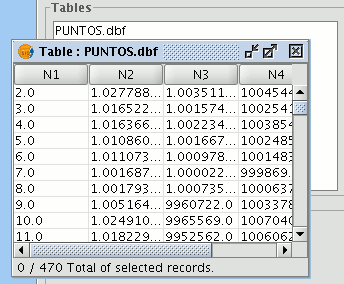
Click on the "See table of attributes" button from the display window of a view with at least one active layer, i.e. a layer that is selected in the ToC,

or go to the "Layer" menu and then select the "See table of attributes" option.
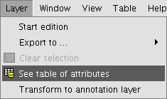
The table will automatically be added to the project.
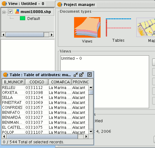
If you minimise the view, go back to the "Project manager" and select "Tables" as the document type, you will see that the table displayed in the view appears in the text box.
Table properties
You can access “Table properties” from the “Project manager” window.
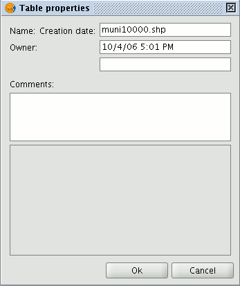
You can use this window to:
- Rename the table.
- Edit the creation date.
- Add an owner to the table.
- Add comments.
When you have input the changes, click on “Ok” and they will be saved.
Table tools
When a table has been loaded, either from the “Project manager” or from the view, the tools associated with the table will appear in the tool bar.

A new menu, called “Table”, will also be activated in the tool bar. This can also be used to access the different tools.
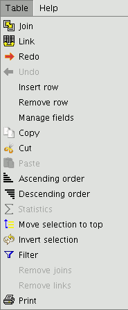
You can access this option by clicking on the following button

or by going to the “Table” menu and then to “Statistics”.
The “Statistics” tool allows you to obtain the most common statistical values.
N.B.: Remember that the tool will not be activated until you select a numerical field.
If you wish to obtain field statistics, select the field (left click on the field heading), then click on the “Statistics” tool.
You can only obtain statistics from a series of records, firstly, select the field the values are located in, then select the desired records, and click on the “Statistics” tool.
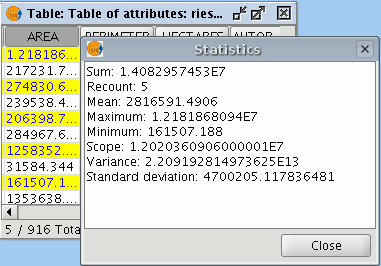
You can access this tool by clicking on the “Filter” button in the tool bar

or by going to the “Table” menu and then to “Filter”. The “Filter” tool works in much the same way as in the “Views” section.
gvSIG allows selections to be made using filters. Selection using filters allows you to define exactly what you want to select, including several attributes, operators and calculations.
Requests can be made using logical operators, such as “equals” “more than” “different from”, etc.
If you press the “Filter” button in the tool bar, a dialogue window will appear to define your request.

Fields: Double click on the field you wish to add to your request from the “Fields” list in the layer.
Logical operators: These allow you to insert a logical expression into your query by clicking on them.
Values: This shows a list with the different values the selected field has. If you wish to add a value to the request, double click on it.
Request: This is the window which represents the request to be made. You can write here directly.
Selection buttons: These buttons make the request using:
- “New set” (deletes any previous selections).
- “Add to set” (adds the elements selected by the query to the existing elements).
- “Select from set” (makes the request from the selected elements).
N.B.: In a gvSIG view, when you activate a layer by selecting it in the ToC, the filter tool will also be activated in the tool bar, even though no table has been loaded. This allows you to work with the table associated with the selected layer. The "Table" menu will also be added in the menu bar. This provides another way to access the filter tool when it drops down.
You can access this tool by clicking on the following tool bar button

or by going to the “Table” menu and then to “Ascending order”.
The “Ascending order” tool allows you to order the table records.
- It orders the values from the lowest to the highest in a numerical field.
- It orders the records in alphabetical order, starting from “A” in a text field.
You can access this tool by clicking on the following tool bar button

or by going to the “Table” menu and then to “Descending order”. The “Descending order” tool allows you to order the table records. It orders the values from the highest to the lowest in a numerical field. It orders the records in alphabetical order, starting from “Z” in a text field.
You can access this tool by clicking on the following button in the tool bar

or by going to the “Table” menu and then to “Link”. The “Link” tool allows two tables to be linked via a common field, so that any changes that take place in one table will also be shown in the other one.
Firstly, specify the source table the link is to be made from.
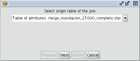
Then specify the field to be used for the link.
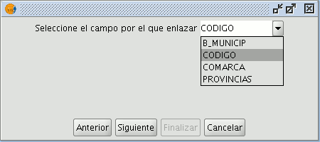
Then indicate the table you wish to link to the first one.
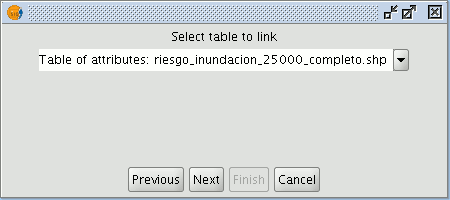
Finally, indicate the field in the second table which is common to the first one.
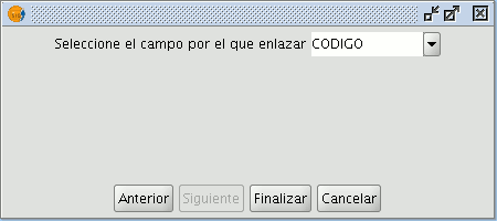
This tool allows the records selected in the table to be moved to the top of the table. You can access this tool by clicking on the following button in the tool bar

or by going to the “Table” menu and then to “Move selection to top”. The following table shows an example in which two records have been selected to move to the top of the table.
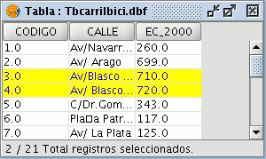
If you click on the button, the table will change the position of the selected records.
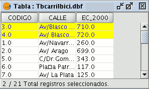
Although .dbf files should contain a byte to indicate character encoding, this information is usually not present. gvSIG provides the Shalom tool that sets the encoding and then reads the information in the table using that encoding. If the encoding is not set in this way then gvSIG will read the table data using the default encoding.
It is possible to set the character encoding of a table by selecting Table > Set encoding to .dbf files from the menu bar. Choose the table for which the encoding needs to be set and then select the encoding type (charset). This encoding setting is recorded permanently in the table.
Now the table can be added to the gvSIG project. When gvSIG opens the table the character encoding is read and the characters in the table are correctly displayed.
Note: The correct display of characters depends not only on the encoding setting, but also on the virtual machine that is installed (specifically Java 1.6, which supports more encodings than Java 1.5).
This option can be accessed by opening the Window > Preferences menu and then selecting DBF default encoding.
gvSIG will use the selected encoding as the default when adding a .dbf file to a project, and will also use it when exporting a table that uses a specific encoding.
The export of a table might not be correct if the character encoding is incorrectly configured in the gvSIG preferences.
Adding a table from csv file
From version 0.5 onwards, gvSIG can read information contained in a plain text file, whose fields are separated by a semi-colon.
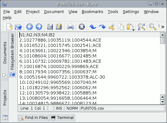
To carry out this operation, go firstly to the “Project manager”. Select “Tables” and then click on “New”. A search dialogue box will open. Click on “Add” and the file browser will appear in a new window (select “csv string” in “Type of file” to show the csv files).
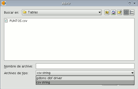
When the .csv file has been selected, click on “Open”.
If you click on “Ok”, the data of the table you have added will be shown.
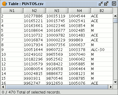
Adding a table from JDBC
The contents of a data base table can be imported to gvSIG using data base managers (PostgreSQL, MySQL, GBMS-HSQLDB, ODBC). gvSIG processes the information obtained just like any other table.
Note: Oracle drivers installation is required for access to Oracle Spatial databases of the geoBD extension. Please follow the steps bellow: Go to Oracle Database 10g Release 2 (10.2.0.3) drivers.
Accept the license terms. In the next page, download the file ojdbc14.jar (1,545,954 bytes) - classes for use with JDK 1.4 and 1.5. (Registration required)
Move this file to the next folder:
- Windows:
Move the file to the:
bin\gvSIG\extensiones\com.iver.cit.gvsig\lib
folder, that is in the directory where gvSIG is installed.
- Linux:
Move the file to the:
bin/gvSIG/extensiones/com.iver.cit.gvsig/lib folder
, that is in the directory where gvSIG is installed.
To load a table with the information obtained from a JDBC data origin you must:
Firstly, go to the "Project manager" and select "Tables". Then click on "New". Select the “Data base” tab in the window that opens (“New table”) and configure the data base server connection parameters:
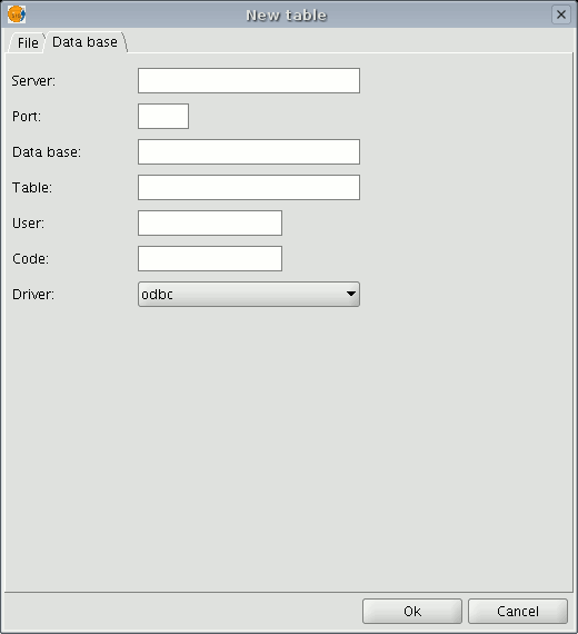
If the information entered is correct, a new table will be created in gvSIG with the information contained in the original JDBC table.
-----------------------------------
